Linear algebra plays a fundamental role in data science. It is used in many areas such as linear regression, principal component analysis (PCA), singular value decomposition (SVD), eigendecomposition, and more. Linear algebra is used to solve systems of linear equations, which are used to model many real-world problems. It is also used to represent and manipulate large sets of data, such as images, videos, and audio. The eigenvectors and eigenvalues of a matrix are used in PCA and SVD, which are key techniques for data compression and dimensionality reduction. Overall, linear algebra provides the mathematical foundation for many data science techniques and is essential for understanding and implementing machine learning algorithms. Some of the key applications of linear algebra in data science are :

1. Linear Regression
2. Principal Component Analysis (PCA)
3. Singular Value Decomposition (SVD)
4. Eigenvalue Decomposition
5. Matrix Factorization
6. Latent Semantic Analysis (LSA)
7. Recommender Systems
8. Neural Networks
9. Computer Vision
10. Natural Language Processing (NLP)
11. Clustering
12. Image Processing
13. Optimization
14. Signal Processing
15. Control Systems.

Let’s understand few in detail.

The most commonly used loss function for linear regression is the Mean Squared Error (MSE) loss function. The MSE loss function measures the average squared difference between the predicted values and the true values. Mathematically, it is defined as:

MSE = (1/n) * Σ(y_i – y_pred_i)^2

where y_i is the true value of the i-th sample, y_pred_i is the predicted value of the i-th sample, and n is the number of samples.

The MSE loss function has some useful properties such as it is differentiable, and it is also a convex function, so it can be minimized by many optimization algorithms.

The goal of linear regression is to find the best parameters that minimize the MSE loss function. In other words, the best parameters minimize the difference between the predicted and true values. The best parameters can be found using optimization algorithms like gradient descent, which iteratively updates the parameters to minimize the MSE loss function. Refer the following figure for same:

It’s also worth mentioning that there are other loss functions that can be used for linear regression like Mean Absolute Error (MAE), Huber loss, etc. The choice of loss function depends on the problem and the data.

In Python, the most popular library for linear regression is scikit-learn. Here’s an example of how to perform linear regression using scikit-learn:

from sklearn.linear_model import LinearRegression
from sklearn.model_selection import train_test_split

# Import your data
X = ...  # independent variables
y = ...  # dependent variable

# Split the data into training and testing sets
X_train, X_test, y_train, y_test = train_test_split(X, y, test_size=0.2)

# Create a LinearRegression object
reg = LinearRegression()

# Fit the model to the training data
reg.fit(X_train, y_train)

# Make predictions on the test set
y_pred = reg.predict(X_test)

The main idea behind PCA is to find a new set of linear combinations of the original features, called principal components (PCs), that capture the most important information in the data. These PCs are chosen such that they are mutually orthogonal (uncorrelated) and ordered by the amount of variance they explain.

The process of PCA can be broken down into the following steps:

1. Standardize the data by subtracting the mean and dividing by the standard deviation.
2. Calculate the covariance matrix of the standardized data.
3. Calculate the eigenvectors and eigenvalues of the covariance matrix. The eigenvectors are the principal components, and the eigenvalues are used to order the components by the amount of variance they explain.
4. Select the top k eigenvectors (principal components) that explain the most variance in the data.
5. Transform the original data into the new PCA space by multiplying the standardized data by the top k eigenvectors.

One of the main benefits of PCA is that it can be used to visualize high-dimensional data in a lower-dimensional space. By reducing the number of features, PCA can also make machine learning algorithms more efficient and improve their performance.

how you can implement PCA in Python using the scikit-learn library:

from sklearn.decomposition import PCA
import numpy as np

# create a sample data set
data = np.random.rand(50, 4)

# create an instance of the PCA class
pca = PCA(n_components=3) # n_components is the number of principal components to keep

# fit the PCA model to the data
pca.fit(data)

# transform the data into the PCA space
pca_data = pca.transform(data)

# access the principal components
print(pca.components_)

This code will create a sample data set with 50 samples and 4 features and then applies PCA to reduce the number of features to 3. The fit() method is used to train the PCA model on the data, and the transform() method is used to transform the data into the PCA space. The principal components are stored in the components_ attribute of the PCA object.

You can also use the fit_transform() method to perform both the fitting and transforming steps in one line:

pca_data = pca.fit_transform(data)

You can also access the explained variance ratio of each component with pca.explained_variance_ratio_

Please note that in this example, the data is not standardized before applying PCA, that is usually a good practice as it makes sure that all features are on the same scale, but for the sake of simplicity, it was not included in the example.

Also, it’s worth noting that this is just a simple example, in real-world problems, the data might be very large or the features might be correlated and it might not be possible to run PCA on the entire dataset, in this case, it is common to use other techniques to reduce dimensionality and to select a subset of features before applying PCA.

It’s worth noting that PCA is not always the best technique for reducing dimensionality and there are other techniques available such as t-SNE, LLE, etc. The choice of technique depends on the problem and the data.

Singular Value Decomposition (SVD) is a powerful tool in linear algebra that is used to decompose a matrix into simpler, more manageable components. It is a factorization of a matrix into a canonical form, which makes it useful for various linear algebraic operations.

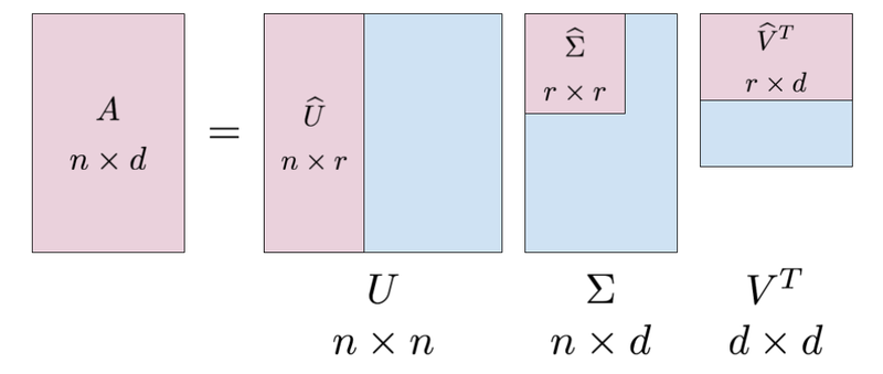
The SVD of a matrix A is represented as A = UΣV*, where U and V are orthogonal matrices and Σ is a diagonal matrix containing the singular values of A.

U is an m x m matrix (where m is the number of rows of A) whose columns are the left singular vectors of A. The columns of U are orthonormal, meaning that they are unit vectors (length 1) and are perpendicular to each other.

Σ is an m x n matrix (where n is the number of columns of A) and is a diagonal matrix whose entries are the singular values of A. These values are always non-negative and are arranged in descending order on the diagonal.

V* is an n x n matrix whose columns are the right singular vectors of A. The columns of V are also orthonormal.

SVD has many applications in linear algebra and beyond. One of the key applications is in data compression. By keeping only a small number of the largest singular values, we can approximate the original matrix A with a low-rank matrix that retains most of the information. SVD is also used in information retrieval and text mining, image processing, and solving linear equations.

In summary, SVD is a powerful technique in linear algebra that allows us to decompose a matrix into simpler and more manageable components. The decomposition is unique and can be used in various linear algebraic operations such as data compression, information retrieval, image processing and solving linear equations.

To calculate the singular value decomposition of a matrix in Python using the NumPy library:

import numpy as np

# Create a matrix
A = np.array([[1, 2], [3, 4], [5, 6]])

# Perform SVD
U, S, V = np.linalg.svd(A)

# Print the results
print("U = \n", U)
print("S = \n", S)
print("V = \n", V)

# Reconstruct the original matrix
A_reconstructed = U @ np.diag(S) @ V
print("Original matrix = \n", A)
print("Reconstructed matrix = \n", A_reconstructed)

In the above code snippet, A is the matrix we are decomposing. The np.linalg.svd() function returns the matrices U, S and V which are orthogonal matrices and a diagonal matrix respectively. The original matrix can be reconstructed by the dot product of U, S, and V respectively. The last two lines of the code snippet, verify the reconstructed matrix A_reconstructed and the original matrix A are identical.

Clustering is a method of grouping similar objects together based on some measure of similarity or distance. In mathematics, clustering is often formulated as an optimization problem, where the goal is to minimize the sum of distances between points in the same cluster and maximize the sum of distances between points in different clusters. Clustering algorithms can be divided into two main categories: hard clustering and soft clustering. Hard clustering algorithms assign each data point to exactly one cluster, while soft clustering algorithms assign each data point to multiple clusters with varying degrees of membership.

Clustering is a technique used in machine learning and statistics to group similar data points together. There are various clustering algorithms available, including:

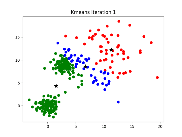
1. K-Means: This is one of the most popular clustering algorithms. It aims to partition a set of n observations into k clusters, where each observation belongs to the cluster with the nearest mean.
2. Hierarchical Clustering: This algorithm creates a hierarchy of clusters by merging or splitting them successively. There are two types of hierarchical clustering: agglomerative and divisive.
3. DBSCAN: Density-Based Spatial Clustering of Applications with Noise. It finds high density areas of the data and expands clusters from those areas.
4. GMM: Gaussian Mixture Model is a probabilistic model that assumes all the data points are generated from a mixture of a finite number of Gaussian distributions with unknown parameters.
5. Spectral Clustering: Spectral Clustering is a technique based on eigenvalue decomposition of the Laplacian matrix of the graph representation of the data.
6. Affinity Propagation: It sends “messages” between data points to cluster them, and it chooses the exemplars that are most representative of other points.
7. Mean Shift: Mean shift clustering aims to discover “blobs” in a smooth density of samples. It is a centroid-based algorithm, or a distance-based algorithm.

K-Means algorithm implementation in python include:

from sklearn.cluster import KMeans
import numpy as np

# Generate sample data
X = np.array([[1, 2], [1, 4], [1, 0], [4, 2], [4, 4], [4, 0]])

# Create a KMeans model with 2 clusters
kmeans = KMeans(n_clusters=2)

# Fit the model to the data
kmeans.fit(X)

# Predict the cluster labels for the data
labels = kmeans.predict(X)

print(labels)

The mathematical solution for a content-based recommender system typically involves creating a feature vector for each item, with the features being the attributes or characteristics of the item. These feature vectors can then be used to compute the similarity between items using a similarity metric such as cosine similarity. Once the similarity between items is calculated, the system can then recommend items that are most similar to the items that the user has liked in the past.

In terms of implementation, a content-based recommender system would typically involve the following steps:

1. Extracting the features of each item, such as genre, director, etc.
2. Creating a feature vector for each item using these extracted features
3. Computing the similarity between items using a similarity metric such as cosine similarity
4. Recommending the most similar items to the user based on their past preferences

In python, libraries such as scikit-learn, pandas, and numpy can be used to implement these steps.

A simple recommender system using Python’s scikit-learn library could look like this:

from sklearn.metrics.pairwise import cosine_similarity
from sklearn.metrics import pairwise_distances

# create a user-item matrix
ratings_matrix = pd.pivot_table(df, values='rating', index='user_id', columns='item_id')

# calculate the cosine similarity between items
item_similarity = cosine_similarity(ratings_matrix.T)

# create a function to get the top n similar items to an item
def get_similar_items(item_id, n):
    item_index = item_id - 1 # the index in the similarity matrix starts at 0
    similar_items = list(enumerate(item_similarity[item_index]))
    similar_items = sorted(similar_items, key=lambda x: x[1], reverse=True)
    similar_items = similar_items[1:n+1] # remove the first item as it is the item itself
    return similar_items

# test the function
get_similar_items(1, 5) # get the top 5 similar items to item 1

It is worth noting that this is a simple example of a content-based recommender system that uses cosine similarity to calculate the similarity between items based on their ratings. Other more complex types of recommenders such as collaborative filtering, matrix factorization and deep learning models are also available.

A sample collaborative filtering using the python library is:

from surprise import Dataset, Reader
from surprise import SVD

# Load the dataset
data = Dataset.load_builtin('ml-100k')

# Use the SVD algorithm
algo = SVD()

# Train the model
trainset = data.build_full_trainset()
algo.fit(trainset)

# Make predictions
uid = str(196)  # raw user id (as in the ratings file). They are **strings**!
iid = str(302)  # raw item id (as in the ratings file). They are **strings**!
pred = algo.predict(uid, iid)
print(pred)

In this example, the dataset used is the built-in MovieLens 100k dataset. The SVD algorithm is used to train the model, and the predict() function is used to make predictions for a specific user and item. This is just one example of how collaborative filtering can be implemented in Python using the surprise library, and there are many other ways it can be implemented using different libraries and algorithms.

A neural network is a mathematical model inspired by the structure and function of the human brain. It is composed of layers of interconnected “neurons,” which process and transmit information. Each neuron receives input from other neurons, performs a mathematical operation on that input, and generates an output. The output of one layer becomes the input for the next layer. The final output of the neural network represents a prediction or decision based on the input it received.

The mathematical foundation of a neural network lies in linear algebra and calculus. Linear algebra is used to manipulate the weight matrices that determine the strength of the connections between neurons, and calculus is used to optimize the parameters of the network to minimize the error in predictions. The most commonly used optimization algorithm is stochastic gradient descent (SGD).

A neural network is trained using a dataset of labeled examples, where the network adjusts the weight matrices to minimize the difference between the predicted output and the true output. The process of training a neural network is also known as backpropagation, which uses calculus to calculate the gradient of the error with respect to the weight matrices and adjust them accordingly.

In summary, the mathematical foundation of a neural network includes linear algebra for manipulating the weight matrices, calculus for optimization and backpropagation, and probability theory for modeling uncertain and random processes.

Sample code in Python to implement a simple Multilayer Perceptron (MLP) neural network using the popular library Keras:

from keras.models import Sequential
from keras.layers import Dense

# Define the model
model = Sequential()
model.add(Dense(10, input_dim=8, activation='relu'))
model.add(Dense(1, activation='sigmoid'))

# Compile the model
model.compile(loss='binary_crossentropy', optimizer='adam', metrics=['accuracy'])

# Fit the model to the training data
model.fit(X_train, y_train, epochs=10, batch_size=32)

This code creates a simple MLP with one hidden layer containing 10 neurons, and an output layer with 1 neuron, using the ReLU activation function for the hidden layer and sigmoid for the output layer. The model is then compiled with a binary cross-entropy loss function and the Adam optimizer, and is fit to the training data using 10 epochs and a batch size of 32.

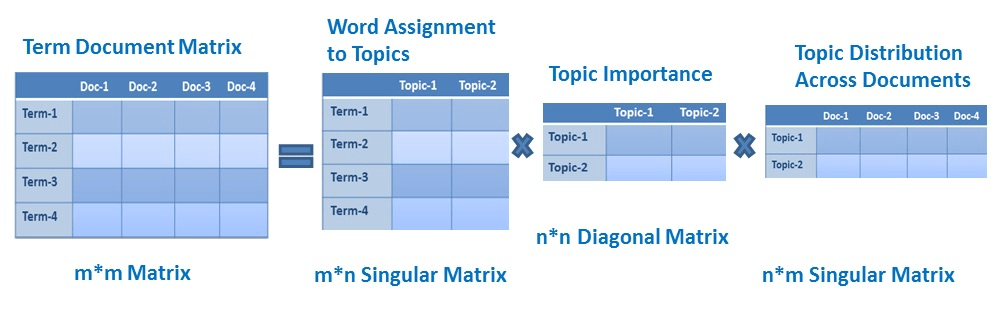
Latent Semantic Analysis (LSA) is a mathematical technique used to analyze and extract the underlying meaning and structure of a collection of text documents. It is based on the idea that words that frequently appear together in a document convey similar meaning.

LSA uses Singular Value Decomposition (SVD) to reduce the dimensionality of a term-document matrix, which represents the frequencies of words in a collection of documents. The goal of LSA is to find a low-dimensional representation of the original matrix that captures the most important relationships between words and documents. In this representation, each word is represented by a vector in a lower-dimensional space, and the similarity between words can be calculated by taking the inner product of their vectors. Additionally, LSA can also be used to discover latent topics in a collection of documents by finding the most important concepts in the reduced matrix.

LSA implementation in Python using the Gensim library:

from gensim import corpora, models

# Define the documents
documents = ["this is the first document",
             "this is the second document",
             "and the third one",
             "is this the first document"]

# Tokenize the documents
texts = [[word for word in document.lower().split()] for document in documents]

# Create a dictionary of words and their integer ids
dictionary = corpora.Dictionary(texts)

# Create a term-document matrix
corpus = [dictionary.doc2bow(text) for text in texts]

# Perform LSA
lsa = models.LsiModel(corpus, id2word=dictionary, num_topics=2)

In this sample code, we first define a list of documents, tokenize them into a list of lists of words, create a dictionary mapping words to integer IDs, and create a term-document matrix. We then use the Gensim library’s LsiModel to perform LSA on the corpus and extract 2 latent topics.

Linear algebra is widely used in computer vision to represent and manipulate images and videos. Some examples of the use of linear algebra in computer vision include:

1. Representation of images: Images can be represented as matrices, where each element of the matrix represents the intensity of a pixel. Linear algebra operations such as matrix multiplication, transposition, and inversion can be used to manipulate and process images.
2. Image processing: Linear algebra techniques such as convolution and filtering can be used to sharpen, blur, and perform other image processing tasks on images.
3. Image recognition: Linear algebra is used to represent and manipulate features of images, which are used in machine learning algorithms to classify images and perform object recognition tasks.
4. Computer vision algorithms such as SIFT, SURF, ORB, etc which are used for feature detection and description, linear algebra plays a key role in them.
5. Camera calibration and 3D reconstruction also heavily rely on Linear Algebra to transform 2D images to 3D coordinates and vice versa.

Overall, linear algebra is an essential tool in the field of computer vision, and its techniques are used to perform a wide range of image processing and analysis tasks.

3D reconstruction is the process of building a 3D model of an object from a set of 2D images or measurements. There are various techniques and algorithms that can be used for 3D reconstruction, such as structure from motion, multi-view stereo, and photogrammetry. The specific sample code for implementing a 3D reconstruction algorithm would depend on the technique being used and the programming language and libraries being employed. However, some common libraries and frameworks used in 3D reconstruction include OpenCV, PCL, and Open3D.

Here is an example of using OpenCV and PCL library in python to perform 3D reconstruction using the structure from motion technique:

import cv2
import open3d as o3d

# Load images
img1 = cv2.imread('image1.jpg')
img2 = cv2.imread('image2.jpg')

# Detect and extract features from images
sift = cv2.xfeatures2d.SIFT_create()
kp1, des1 = sift.detectAndCompute(img1, None)
kp2, des2 = sift.detectAndCompute(img2, None)

# Match features
bf = cv2.BFMatcher()
matches = bf.knnMatch(des1, des2, k=2)

# Filter matches
good = []
for m,n in matches:
    if m.distance < 0.75*n.distance:
        good.append(m)

# Extract matching points
pts1 = np.float32([kp1[m.queryIdx].pt for m in good]).reshape(-1,1,2)
pts2 = np.float32([kp2[m.trainIdx].pt for m in good]).reshape(-1,1,2)

# Compute fundamental matrix
F, mask = cv2.findFundamentalMat(pts1, pts2, cv2.FM_RANSAC)

# Compute essential matrix
E = K.T @ F @ K

# Decompose essential matrix
R1, R2, t = cv2.decomposeEssentialMat(E)

# Compute projection matrices
P1 = np.hstack((np.eye(3,3), np.zeros((3,1))))
P2 = np.hstack((R, t))

# Triangulate points
points_4d_hom = cv2.triangulatePoints(P1, P2, pts1.T, pts2.T)
points_4d = points_4d_hom / np.tile(points_4d_hom[-1, :], (4, 1))
points_3d = points_4d[:3, :].T

# Convert to PointCloud
pcd = o3d.geometry.PointCloud()
pcd.points = o3d.utility.Vector3dVector(points_3d)

# Visualize
o3d.visualization.draw_geometries([pcd])

Please keep in mind that this is a simple example, and in real world applications, the code would be much more complex and would require more steps to be taken for better results.