Lets find the solution by combining dots.

Solution Dots:

Dot 1 : is PCA based on SVD?

Yes, Principal Component Analysis (PCA) is based on the Singular Value Decomposition (SVD) method.

PCA is a technique used to reduce the dimensionality of a data set while preserving as much of the variation in the data as possible. It does this by identifying the directions in the data that have the most variance and projecting the data onto a lower-dimensional subspace along those directions.

SVD is a mathematical technique that decomposes a matrix into three separate matrices, one of which represents the principal components of the original matrix. When PCA is applied to a data set, it is essentially finding the SVD of the data’s covariance matrix and then using the principal components from the SVD to project the data onto a lower-dimensional subspace.

SVD can be used for other purposes as well, such as solving linear equations and finding the rank of a matrix, but when it comes to PCA it is used as a way to decompose a matrix and identify the principal components, which are then used to reduce the dimensionality of the data.

Dot 2: is SVD based on Matrix Diagonalization?

Yes, Singular Value Decomposition (SVD) can be thought of as a generalization of matrix diagonalization.

Matrix diagonalization is a technique used to transform a matrix into a diagonal matrix, which is a matrix with all non-diagonal elements equal to zero. This is achieved by finding a set of eigenvectors for the matrix and transforming the matrix into a new basis set consisting of those eigenvectors.

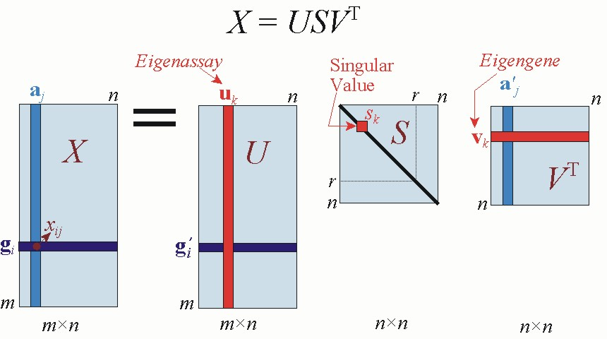
SVD is a more general method that decomposes a matrix into three separate matrices, one of which is a diagonal matrix. Specifically, SVD decomposes a matrix A into the product of three matrices: U, Sigma, and V^T. Where U and V are unitary matrices and Sigma is a diagonal matrix containing the singular values of A.

SVD can be considered as a generalization of matrix diagonalization in the sense that it also decomposes a matrix into simpler form, but it also decomposes a matrix into two unitary matrices, which are not always diagonal, and a diagonal matrix (sigma) containing the singular values of A.

Therefore, while matrix diagonalization is a special case of SVD in that it finds the eigenvectors of a matrix and decomposes it into a diagonal matrix, SVD is a more general method that can be applied to any matrix, even non-square matrices, and decomposes it into a combination of unitary matrices and a diagonal matrix.

Dot 3 : is matrix diagonalization based on eigen values and eigen vectors?

Yes, matrix diagonalization is based on eigenvalues and eigenvectors.

A matrix can be diagonalized by a change of basis that brings it into a new set of coordinates where the matrix is represented by a diagonal matrix. A matrix A is diagonalizable if and only if there exists a set of non-zero vectors, called eigenvectors, and scalars, called eigenvalues, such that:

Av = lambda v

Where v is an eigenvector and lambda is the corresponding eigenvalue. The eigenvectors of a matrix are the vectors that are unchanged after the matrix transformation. The eigenvalues are scalars that define the amount of stretching or shrinking that occurs along the eigenvectors.

Matrix diagonalization can be performed by finding the eigenvectors and eigenvalues of the matrix and transforming it into a new basis set consisting of those eigenvectors. This is often a useful step when solving differential equations or when studying the properties of a matrix, such as its stability or its transformation properties.

In summary, matrix diagonalization is the process of finding eigenvectors and eigenvalues of a matrix and transforming it into a new basis set consisting of those eigenvectors, such that the matrix is represented by a diagonal matrix, which makes it easier to analyze the matrix’s properties.

Dot 4: Vectorization of matrix

Vectorization of a matrix refers to the process of converting a matrix into a single vector (1-dimensional array) by arranging its elements in a specific order. This is often done in order to simplify the representation of the matrix and make it more efficient to work with, as well as to perform linear algebra operations such as dot products and matrix-vector multiplications.

There are a few different ways to vectorize a matrix, depending on the specific application and the desired outcome.

• Row-wise vectorization: In this method, the elements of the matrix are arranged in the vector in the same order as they appear in the rows of the matrix. This is also called flattening the matrix.
• Column-wise vectorization: In this method, the elements of the matrix are arranged in the vector in the same order as they appear in the columns of the matrix.
• Diagonal-wise vectorization: In this method, the elements of the matrix are arranged in the vector by taking the diagonal elements of the matrix.

The process of vectorization is often used in machine learning and data analysis, where matrices are used to represent large sets of data and need to be processed efficiently. In addition, some libraries and optimization algorithms also require vectorized data for efficient computations.

It is also worth to mention that sometimes the term vectorization is used to refer to the process of using vector operations (such as dot products and matrix-vector multiplications) to perform calculations on matrices in a more efficient way, rather than using loops or nested loops. This is also known as vectorized computation.

Dot 5 : The bridge between linear algebra(LA) and vector calculus(VC)

Linear algebra and vector calculus are two branches of mathematics that are closely related and often used together.

Linear algebra deals with the properties and operations of vectors and matrices, and is often used to represent and manipulate linear systems of equations. It also provides mathematical tools to analyze the properties of linear transformations and eigenvalues, eigenvectors and orthonormal bases.

Vector calculus, on the other hand, deals with the properties and operations of vector fields, which are functions that assign a vector to every point in a space. Vector calculus is used to study vector-valued functions, such as velocity and acceleration, and provides mathematical tools for analyzing the properties of vector fields, such as gradient, divergence, and curl.

The bridge between linear algebra and vector calculus is the idea of representing a vector field with a matrix. The matrix can be used to represent the linear transformation and the vector calculus can be used to study the properties of the transformed vector field.

For example, in physics, the position, velocity, and acceleration of a particle moving in space can be represented by a vector field. The linear transformation of the position vector is given by the velocity vector and the linear transformation of the velocity vector is given by the acceleration vector. The linear algebra provides the mathematical tools to analyze these linear transformations, and the vector calculus provides the mathematical tools to study the properties of these vector fields, such as the gradient, divergence, and curl.

In summary, linear algebra and vector calculus are related and complementary branches of mathematics. Linear algebra provides the mathematical tools to represent and analyze linear systems of equations and the properties of linear transformations. Vector calculus provides the mathematical tools to study the properties of vector fields and their transformations. Together, they provide a powerful mathematical framework for analyzing and understanding a wide range of physical and engineering systems.