Basic Indexing and Slicing

NumPy array indexing is a rich topic, as there are many ways you may want to select a subset of your data or individual elements. One-dimensional arrays are simple; on the surface they act similarly to Python lists:

In [1]: arr = np.arange(10)
In [2]: arr
Output: array([0, 1, 2, 3, 4, 5, 6, 7, 8, 9])
In [3]: arr[5]
Output: 5
In [4]: arr[5:8]
Output: array([5, 6, 7])
In [5]: arr[5:8] = 12
In [6]: arr
Output: array([ 0, 1, 2, 3, 4, 12, 12, 12, 8, 9])

As you can see, if you assign a scalar value to a slice, as in arr[5:8] = 12, the value is propagated (or broadcasted henceforth) to the entire selection. An important first distinction from Python’s built-in lists is that array slices are views on the original array. This means that the data is not copied, and any modifications to the view will be reflected in the source array.
To give an example of this, I first create a slice of arr:

In [7]: arr_slice = arr[5:8]
In [8]: arr_slice
Output: array([12, 12, 12])

Now, when I change values in arr_slice, the mutations are reflected in the original array arr:

In [9]: arr_slice[1] = 12345
In [10]: arr
Output: array([ 0, 1, 2, 3, 4, 12, 12345, 12, 8,
 9])

The “bare” slice [:] will assign to all values in an array:

In [11]: arr_slice[:] = 64
In [12]: arr
Output: array([ 0, 1, 2, 3, 4, 64, 64, 64, 8, 9])

If you are new to NumPy, you might be surprised by this, especially if you have used other array programming languages that copy data more eagerly. As NumPy has been designed to be able to work with very large arrays, you could imagine performance and memory problems if NumPy insisted on always copying data.

With higher dimensional arrays, you have many more options. In a two-dimensional array, the elements at each index are no longer scalars but rather one-dimensional arrays:

In [13]: arr2d = np.array([[1, 2, 3], [4, 5, 6], [7, 8, 9]])
In [14]: arr2d[2]
Output: array([7, 8, 9])

Thus, individual elements can be accessed recursively. But that is a bit too much work, so you can pass a comma-separated list of indices to select individual elements. So these are equivalent:

In [15]: arr2d[0][2]
Output: 3
In [16]: arr2d[0, 2]
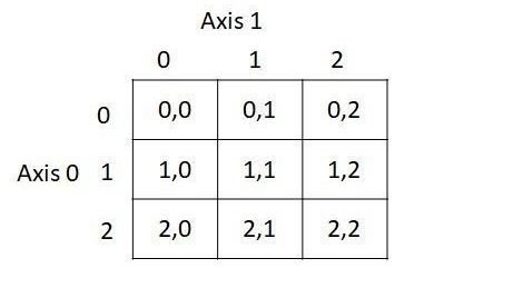
Output: 3

I find it helpful to think of axis 0 as the “rows” of the array and axis 1 as the “columns.”

In multidimensional arrays, if you omit later indices, the returned object will be a lower dimensional ndarray consisting of all the data along the higher dimensions. So in the 2 × 2 × 3 array arr3d:

In [17]: arr3d = np.array([[[1, 2, 3], [4, 5, 6]], [[7, 8, 9], [10, 11, 12]]])
In [18]: arr3d
Output: array([[[ 1,  2,  3],
                [[4,  5,  6]],
                [[ 7,  8,  9],
                 [10, 11, 12]]])

arr3d[0] is a 2 × 3 array:

In [19]: arr3d[0]
Output: array([[1, 2, 3],
               [4, 5, 6]])

Both scalar values and arrays can be assigned to arr3d[0]:

In [20]: old_values = arr3d[0].copy()
In [21]: arr3d[0] = 42
In [22]: arr3d
Output:
 array([[[42, 42, 42],
                 [42, 42, 42]],
                [[ 7, 8, 9],
                 [10, 11, 12]]])
In [23]: arr3d[0] = old_values
In [24]: arr3d
Output: 
array([[[ 1, 2, 3],
                [ 4, 5, 6]],
               [[ 7, 8, 9],
                [10, 11, 12]]])

Similarly, arr3d[1, 0] gives you all of the values whose indices start with (1, 0), forming a 1-dimensional array:

In [25]: arr3d[1, 0]
Output: array([7, 8, 9])

This expression is the same as though we had indexed in two steps:

In [26]: x = arr3d[1]
In [27]: x
Output: 
array([[ 7, 8, 9],
      [10, 11, 12]])
In [28]: x[0]
Output: array([7, 8, 9])

Note that in all of these cases where subsections of the array have been selected, the returned arrays are views.

Indexing with slices

Like one-dimensional objects such as Python lists, ndarrays can be sliced with the familiar syntax:

In [29]: arr
Output: array([ 0, 1, 2, 3, 4, 64, 64, 64, 8, 9])
In [30]: arr[1:6]
Output: array([ 1, 2, 3, 4, 64])

Consider the two-dimensional array from before, arr2d. Slicing this array is a bit different:

In [31]: arr2d
Output: 
array([[1, 2, 3],
       [4, 5, 6],
       [7, 8, 9]])
In [32]: arr2d[:2]
Output: array([[1, 2, 3],
               [4, 5, 6]])

As you can see, it has sliced along axis 0, the first axis. A slice, therefore, selects a range of elements along an axis. It can be helpful to read the expression arr2d[:2] as “select the first two rows of arr2d.”
You can pass multiple slices just like you can pass multiple indexes:

In [33]: arr2d[:2, 1:]
Output: array([[2, 3],
               [5, 6]])

When slicing like this, you always obtain array views of the same number of dimensions. By mixing integer indexes and slices, you get lower dimensional slices.
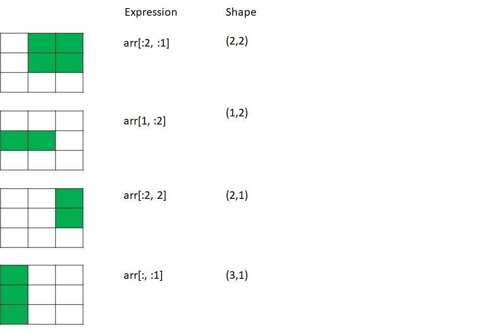
For example, I can select the second row but only the first two columns like so:

In [34]: arr2d[1, :2]
Out[put: array([4, 5])

Similarly, I can select the third column but only the first two rows like so:

In [35]: arr2d[:2, 2]
Output: array([3, 6])

Note that a colon by itself means to take the entire axis, so you can slice only higher dimensional axes by doing:

In [36]: arr2d[:, :1]
Output: array([[1],
               [4],
               [7]])

Of course, assigning to a slice expression assigns to the whole selection:

In [37]: arr2d[:2, 1:] = 0
In [38]: arr2d
Output: array([[1, 0, 0],
               [4, 0, 0],
               [7, 8, 9]])