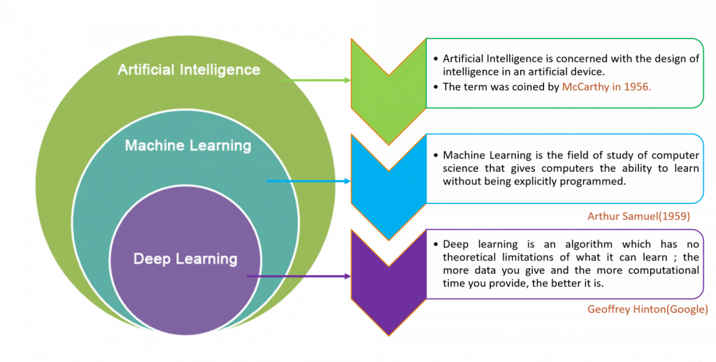
A Quick Refresher on Machine Learning
ML is the subfield of Artificial Intelligence. As a child learns by examples or seeing and tagging names of things, similarly machine learns by seeing/ understanding several examples. A innocent child need a few examples to learn something whereas a machine needs many more to get an idea.
Machine Learning QnA
Question: 1 What are the most important machine learning techniques?
Answer:
In his famous essay “Computing Machinery and Intelligence” Alan Turing asked a fundamental question “Can machines do what we (as thinking entities) can do?” Machine learning is not about thinking but more about a related activity: Learning or better, according to Arthur Samuel, the “Field of study that gives computers the ability to learn without being explicitly programmed”. Machine learning techniques are typically classified into two categories: In supervised learning pairs of examples made up by (inputs, desired output) are available and the computer learns a model according to which given an input, a desired output with a minimal error is predicted. Classification, Neural Networks and Regression are all examples of supervised learning. For all techniques we assume that there is an oracle or a teacher that can teach to computers what to do in order for them to apply the learned lessons on new unseen data. In unsupervised learning computers have no teachers and they are left alone in searching for structures, patterns and anomalies in data. Clustering and Density Estimations are typical examples of unsupervised machine learning. Let us now review the main machine learning techniques: In classification the teacher presents pairs of (inputs, target classes) and the computer learns to attribute classes to new unseen data. Naïve Bayesian, SVM, Decision Trees and Neural Networks are all classification methodologies. The first two are discussed in this volume, while the remaining ones will be part of the next volume. In Regression the teacher presents pairs of (inputs, continuous targets) and computers learn how to predict continuous values on new and unseen data. Linear and Logistic regression are examples which will be discussed in the present volume. Decision Trees, SVM and Neural Networks can also be used for Regression. In Associative rule learning computers are presented with a large set of observations, all being made up of multiple variables. The task is then to learn relations between variables such us A & B C (if A and B happen, then C will also happen). In Clustering computers learn how to partition observations in various subsets, so that each partition will be made up of similar observations according to some well-defined metric. Algorithms like K-Means and DBSCAN belong also to this class. In Density estimation computers learn how to find statistical values that describe data. Algorithms like Expectation Maximization belong also to this class
Question: 2 Why are Features extraction and engineering so important in machine learning?
Answer:
The Features are the selected variables for making predictions. For instance, suppose you’d like to forecast whether tomorrow there will be a sunny day then you will probably pick features like humidity (a numerical value), speed of wind (another numeric value), some historical information (what happened during the last few years), whether or not it is sunny today (a categorical value yes/no) and a few other features. Your choice can dramatically impact on your model for the same algorithm and you need to run multiple experiments in order to find what the right amount of data and what the right features are in order to forecast with minimal error. It is not unusual to have problems represented by thousands of features and combinations of them and a good feature engineer will use tools for stack ranking features according to their contribution in reducing the error for prediction. Different authors use different names for different features including attributes, variables and predictors. In this book we consistently use features. Features can be categorical such as marital status, gender, state of residence, place of birth, or numerical such as age, income, height and weight. This distinction is important because certain algorithms such as linear regression work only with numerical attributes and if categorical features are present, they need to be somehow encoded into numerical values. In other words, feature engineering is the art of extracting, selecting and transforming essential characteristics representing data. It is sometimes considered less glamourous than machine learning algorithms but in reality any experienced Data Scientist knows that a simple algorithm on a well-chosen set of features performs better than a sophisticated algorithm on a not so good set of features. Also simple algorithms are frequently easier to implement in a distributed way and therefore they scale well with large datasets. So the rule of thumb is in what Galileo already said many centuries ago: “Simplicity is the ultimate sophistication”. Pick your algorithm carefully and spend a lot of time in investigating your data and in creating meaningful summaries with appropriate feature engineering. Real world objects are complex and features are used to analytically represent those objects. From one hand this representation has an inherent error which can be reduced by carefully selecting a right set of representatives. From the other hand we might not want to create a too complex representation because it might be computationally expensive for the machine to learn a sophisticate model, indeed such model could possibly not generalize well to the unseen data. Real world data is noisy. We might have very few instances (outliers) which show a sensible difference from the majority of the remaining data, while the selected algorithm should be resilient enough to outliers. Real world data might have redundant information. When we extract features, we might be interested in optimizing simplicity of learned models and discard new features which show a high correlation with the already observed ones. ETL is the process of Extraction, Transformation and Loading of features from real data for creating various learning sets. Transformation in particular refers to operations such as features weighting, high correlated features discarding, the creation of synthetic features derivative of the one observed in the data and the reduction of high dimension features space into a lower one by using either hashing or rather sophisticate space projection techniques. For example in this book we discuss:
- TFxIDF, an example of features weighting used in text classification
- ChiSquare, an example of filtering of highly correlated features
- Kernel Trick, an example of creation of derivative features
- Hashing, a simple technique to reduce feature space dimensions
- Binning, an example of transformation of continuous features into a discrete one. New synthetic features might be created in order to represent the bins.
Question: 3 Can you provide an example of features extraction?
Answer:
Let’s suppose that we want to perform machine learning on textual files. The first step is to extract meaningful feature vectors from a text. A typical representation is the so called bag of words where: a) Each word in the text collection is associated with a unique integer assigned to it. b) For each document , the number of occurrences of each word is computed and this value is stored in a matrix. Please, note that is typically a sparse matrix because when a word is not present in a document, its count will be zero. NumPy, Scikit-learn and Spark all support sparse vectors. Let’s see an example where we start to load a dataset made up of Usenet articles where the alt. atheism category is considered and the collection of text documents is converted into a matrix of token counts. We then print the .
from sklearn.datasets import fetch_20newsgroups
from sklearn.feature_extraction.text
import CountVectorizer
categories =['alt.atheism']
newsgroups_train = fetch_20newsgroups(subset='train', categories=categories)
count_vect = CountVectorizer() Train_counts =
count_vect.fit_transform(newsgroups_train.data) print
count_vect.vocabulary_.get(u'man')
Question: 4 What is a training set, a validation set, a test set and a gold set in supervised and unsupervised learning?
Answer:
In machine learning a set of true labels is called the gold set. This set of examples is typically built manually either by human experts or via crowdsourcing with tools like the Amazon Mechanical Turk or via explicit/implicit feedback collected by users online. For instance: a gold set can contain news articles that are manually assigned to different categories by experts of the various subjects, or it might contain movies with associated rating provided by Netflix users, or ratings of images collected via crowdsourcing.
Supervised machine learning consists of four phases
- Training phase: A sample extracted by the gold set is used to learn a family of data models. Each model can be generated from this family by choosing an appropriate set of hyper-parameters, i.e. factors which can be used for algorithms fine-tuning s;
- Validation phase: The best learned model is selected from the family by picking hyper-parameters which minimize a computed error function on a gold set sample called “validation set”; This phase is used for identifying the best configuration for a given algorithm;
- Test phase: The error for the best learned model is evaluated on a gold set sample called “test set”. This phase is useful for comparing models built by adopting different algorithms;
- Application phase: The learned model is applied to the real-world data.
Two additional observations can be here highlighted: first, the training set, the validation set and the test set are all sampled from the same gold set but those samples are independent. Second, it has been assumed that the learned model can be described by means of two different functions and combined by using a set of hyper-parameters .
Unsupervised machine learning consists in tests and application phases only because there is no model to be learned a-priori. In fact unsupervised algorithms adapt dynamically to the observed data.
Question: 5 What is a Bias – Variance tradeoff?
Answer:
Bias and Variance are two independent sources of errors for machine learning which prevent algorithms to generalize the models learned beyond the training set.
- Bias is the error representing missing relations between features and outputs. In machine learning this phenomenon is called underfitting.
- Variance is the error representing sensitiveness to small training data fluctuations. In machine learning this phenomenon is called overfitting.
A good learning algorithm should capture patterns in the training data (low bias), but it should also generalize well with unseen application data (low variance). In general, a complex model can show low bias because it captures many relations in the training data and, at the same time, it can show high variance because it will not necessarily generalize well. The opposite happens with models with high bias and low variance. In many algorithms an error can be analytically decomposed in three components: bias, variance and the irreducible error representing a lower bound on the expected error for unseen sample data. One way to reduce the variance is to try to get more data or to decrease the complexity of a model. One way to reduce the bias is to add more features or to make the model more complex, as adding more data will not help in this case. Finding the right balance between Bias and Variance is an art that every Data scientist must be able to manage.
Question: 6 What is a cross-validation and what is an overfitting?
Answer:
Learning a model on a set of examples and testing it on the same set is a logical mistake because the model would have no errors on the test set but it will almost certainly have a poor performance on the real application data. This problem is called overfitting and it is the reason why the gold set is typically split into independent sets for training, validation and test. An example of random split is reported in the code section, where a toy dataset with diabetics’ data has been randomly split into two parts: the training set and the test set.
Given a family of learned models, the validation set is used for estimating the best hyper-parameters. However, by adopting this strategy there is still the risk that the hyper-parameters overfit a particular validation set.
The solution to this problem is called cross-validation. The idea is simple: the test set is split in smaller sets called folds and the model is then learned on folds, while the remaining data is used for validation. This process is repeated in a loop and the metrics achieved for each iteration are averaged. An example of cross validation is reported in the section below where our toy dataset is classified via SVM and accuracy is computed via cross-validation. SVM is a classification technique and “accuracy” is a quality measurement (the number of correct predictions made, divided by the total number of predictions made and multiplied by 100 to turn it into a percentage).
Stratified KFold is a variation of k-fold where each set contains approximately the same balanced percentage of samples for each target class as the complete set.
import numpy as np from sklearn
import cross_validation from sklearn
import datasets from sklearn
import svm diabets = datasets.load_diabetes()
X_train, X_test, y_train, y_test = cross_validation.train_test_split(
diabets.data, diabets.target, test_size=0.2, random_state=0)
print X_train.shape, y_train.shape # test size 20%
print X_test.shape, y_test.shape clf = svm.SVC(kernel='linear', C=1) scores = cross_validation.cross_val_score(clf, diabets.data, diabets.target, cv=4) # 4-folds print scores print("Accuracy:%0.2f (+/- %0.2f)" % (scores.mean(), scores.std()))
Question: 7 What are percentiles and quartiles?
A percentile is a metric indicating a value, below which a given percentage of observations falls. For instance: the 50th percentile is the median of a vector of observations; the 25th percentile is the first quartile, the 50th percentile is the second and the 75th percentile is the third one. When the time to provide a service is considered, the 90th , the 95th and the 99th percentiles are generally reported. Percentiles are more resilient than mathematical averages to the contribution of the so-called outliers, e.g. data points that are significantly spread out by the majority of the observations.
import numpy as np x = np.array([0, 1, 4, 5, 6, 8, 8, 9, 11, 10, 19, 19.2, 19.7, 3])
for i in [75, 90, 95, 99]:
print i, np.percentile(x, i)
Question: 8 What is “features hashing”? And why is it useful for BigData?
Answer:
If the space of features is high dimensional, one way to reduce dimensionality is via hashing. For instance: we might combine two discrete but sparse features into one and only denser discrete synthetically created feature by transforming the original observations. This transformation introduces an error because it suffers from potential hash collisions, since different raw features may become the same term after hashing.
However this model might be more compact and, in some situations, we might decide to trade off this risk either for simplicity or because this is the only viable option to handle very large datasets (Big Data).
More sophisticate forms of hashing such as Bloom Filters, Count Min[1]Sketches, minHash and Local Sensitive Hashing are more advanced techniques which will be discussed in the next volume.