Table of Contents

1. Fundamentals

a. Experiment:

An experiment (or trial) is any procedure or action that produces a definite outcome. For instance, rolling a die is an experiment because the result is uncertain until the die lands and shows a face.

b. Sample Space:

The sample space, often denoted as S or Ω, is the set of all possible outcomes of an experiment. For the dice roll experiment, the sample space is ( S = {1, 2, 3, 4, 5, 6} ).

c. Event:

An event is a specific outcome or combination of outcomes from the sample space. It’s essentially a subset of the sample space. For example, in a dice roll, the event “rolling an even number” corresponds to the subset ( E = {2, 4, 6} ).

d. Probability:

Probability measures the likelihood of an event occurring and is always between 0 and 1 (inclusive). The probability of an impossible event is 0, and the probability of a certain event is 1. For a fair dice roll, the probability of rolling a 3, ( P(3) ), is 16.

Problem:

Suppose you draw a card from a standard deck of 52 playing cards. What is the probability that the card is a red Queen?

Given:

There are 2 red Queens in the deck (Queen of Hearts and Queen of Diamonds).
There are 52 cards in total.

Solution:

Let’s define our event:

( A ) is the event that a card drawn is a red Queen.

We want to find the probability ( P(A) ), which is the probability of drawing a red Queen.

The formula for probability is:

$$P(A) = \frac{\text{Number of favorable outcomes}}{\text{Total number of outcomes}}$$

In this case:

$$P(A) = \frac{2}{52}$$

Let’s compute ( P(A) ).

The probability ( P(A) ) is approximately ( 0.0385 ).

This means that if you draw a card from a standard deck, there’s a ( 0.0385 ) (or 3.85%) chance that the card is a red Queen. This result is intuitive because there are 52 cards in total and only 2 of them are red Queens.

2. Conditional Probability and Independence:

a. Conditional Probability:

This is the probability of an event occurring given that another event has already occurred. The conditional probability of event ( A ) given that event ( B ) has occurred is denoted as P(A|B)and is defined as:

$$P(A|B) = \frac{P(A \cap B)}{P(B)}$$

where $$ P(B) \neq 0 $$.

For instance, if we have a deck of cards and we want to find the probability of drawing an Ace given that we’ve drawn a red card, we’d use the formula above.

b. Independence:

Two events ( A ) and ( B ) are said to be independent if the occurrence of one event does not influence the occurrence of the other. For independent events:

$$P(A \cap B) = P(A) \times P(B)$$

If this equation holds true, ( A ) and ( B ) are independent. If not, they are dependent. For instance, if you roll a die and flip a coin, the outcome of the die roll and the outcome of the coin flip are independent events.

Sure! Let’s explore conditional probability with a classic example involving a deck of playing cards.

Problem:

Suppose you draw a card from a standard deck of 52 playing cards. What is the probability that the card is a King, given that it is a face card?

Given:

There are 4 Kings in the deck.
There are 12 face cards in total (4 Kings, 4 Queens, and 4 Jacks).

Solution:

First, let’s define our events:

( A ) is the event that a card drawn is a King.
( B ) is the event that a card drawn is a face card.

We want to find the conditional probability ( P(A|B) ), which is the probability of drawing a King given that we’ve drawn a face card.

Using the formula for conditional probability:

$$P(A|B) = \frac{P(A \cap B)}{P(B)}$$

P(A∩B) is the probability that the card is both a King and a face card. Since every King is a face card, P(A∩B)=P(A).
P(B) is the probability that the card is a face card.

Plugging in the given information:

$$P(A|B) = \frac{\frac{4}{52}}{\frac{12}{52}}$$

Let’s compute P(A|B).

The conditional probability P(A|B) is approximately ( 0.3333 ) or 1/3.

This means that if you’ve drawn a face card from a standard deck, there’s a 1/3 chance that the card is a King. This result makes intuitive sense, as there are three types of face cards (King, Queen, Jack), and they are all equally likely to be drawn.

Understanding Joint Probability

Probability theory is a fundamental concept in mathematics and statistics, playing a crucial role in various real-world applications. One of the key aspects of probability theory is joint probability, which deals with the likelihood of multiple events occurring simultaneously. In this blog post, we will explore the concept of joint probability, its formula, distribution, and provide practical examples to illustrate its significance.

Formula for Joint Probability:

The joint probability of two events ( A ) and ( B ) happening together is denoted as ( P(A \cap B) ) and can be calculated using the formula:

$$P(A \cap B) = P(A) \times P(B|A)$$

This formula represents the probability of event ( A ) occurring multiplied by the conditional probability of event ( B ) occurring given that event ( A ) has occurred.

Joint Probability Distribution:

In probability theory, a joint probability distribution describes the probabilities of different combinations of outcomes for multiple random variables. For discrete variables, it’s a table or a function, and for continuous variables, it’s represented as a joint probability density function (PDF).

Example:

Consider rolling a fair six-sided die (Event ( A )) and flipping a fair coin (Event ( B )). The joint probability of rolling an even number and getting heads can be calculated as follows:

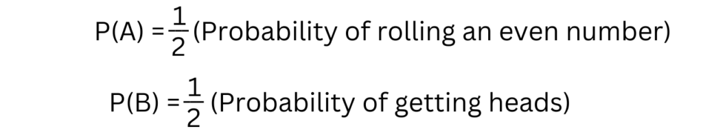
Joint Probability $$P(A \cap B) )) ( = \frac{1}{2} \times \frac{1}{2} = \frac{1}{4} ) or 0.25.$$

Bayes’ Theorem

Probability theory, a cornerstone of mathematics, has given rise to several powerful concepts that find applications in diverse fields, from statistics to artificial intelligence. One such concept that holds immense significance is Bayes’ Theorem. Named after the Reverend Thomas Bayes, this theorem provides a way to update probabilities when new evidence becomes available. It’s a fundamental tool in statistics and has wide-ranging implications in real-world scenarios.

$$P(A|B) = \frac{P(B|A) \times P(A)}{P(B)}$$

Real-Life Applications:

Bayes’ Theorem finds applications in various fields, such as:

Medical Diagnosis: Calculating the probability of a disease given certain symptoms and test results.
Spam Filtering: Determining the probability of an email being spam based on certain keywords.
Finance: Assessing the likelihood of an investment being profitable given market conditions.

Certainly! Bayes’ Theorem is a powerful tool used in various fields, including forensics, to calculate the probability of an event based on prior knowledge and evidence. Here’s a specific use case scenario for Bayes’ Theorem in forensics:

Use Case Scenario: DNA Evidence in Forensics

Imagine a crime scene investigation where DNA evidence is collected. The forensic team is trying to determine the probability that a suspect, let’s call him John, was present at the crime scene based on the DNA evidence found. They have two main pieces of information:

Prior Probability

The probability of a random person being at the crime scene, denoted as P(Crime Scene). This might be a very small number because the crime scene is a specific location, and the chance of a random person being there is low.

Likelihood Ratio

The likelihood ratio (LR) represents how much more likely the observed evidence (DNA) is under the hypothesis that John was at the crime scene (Hypothesis H₁) compared to the hypothesis that he was not (Hypothesis H₂). This ratio is calculated based on the DNA match statistics and the rarity of the DNA profile found.

Using Bayes’ Theorem, the forensic team can calculate the Posterior Probability – the probability that John was at the crime scene given the DNA evidence. Bayes’ Theorem is expressed as follows:

$$P(H₁|E) = \frac{P(E|H₁) \times P(H₁)}{P(E)}$$

Where:

P(H₁|E) is the posterior probability that John was at the crime scene given the evidence (DNA).
P(E|H₁) is the likelihood of finding the observed DNA evidence given that John was at the crime scene.
P(H₁) is the prior probability that John was at the crime scene.
P(E) is the total probability of finding the observed DNA evidence, calculated as P(E|H₁) \times P(H₁) + P(E|H₂) \times P(H₂) , where P(H₂) is the prior probability that John was not at the crime scene.

By plugging in the known values, the forensic team can use Bayes’ Theorem to calculate the probability that John was at the crime scene based on the DNA evidence. This analysis helps legal authorities make more informed decisions about the suspect’s involvement in the crime.

The Extended Bayes’ Theorem

The Extended Bayes’ Theorem allows us to update our beliefs about a hypothesis ((H)) in light of new evidence ((E)) and background knowledge (B). It can be expressed as follows:

$$P(H|E, B) = \frac{P(E|H, B) \times P(H|B)}{P(E|B)}$$

Here’s what each term represents:

P(H|E, B): Posterior probability of hypothesis (H) given evidence (E) and background knowledge (B).
P(E|H, B): Likelihood of observing evidence (E) given that (H) is true, considering background knowledge (B).
P(H|B): Prior probability of hypothesis (H) based on background knowledge (B).
P(E|B): Total probability of observing evidence (E) considering all possible hypotheses and background knowledge (B).

Solve With The Extended Bayes’ Theorem

Extended Bayes’ Theorem is a generalization of Bayes’ Theorem that can handle multiple hypotheses. In the context of forensics with DNA evidence, let’s consider the Extended Bayes’ Theorem to calculate the probability that a specific suspect, John, was at the crime scene based on the DNA evidence.

Extended Bayes’ Theorem is expressed as follows:

$$P(H_i|E) = \frac{P(E|H_i) \times P(H_i)}{\sum_{j=1}^{n} P(E|H_j)}\times P(H_j)$$

Where:

P(H_i|E) is the posterior probability that hypothesis (H_i) is true given the evidence (DNA).
P(E|H_i) is the likelihood of finding the observed DNA evidence given hypothesis (H_i).
P(H_i) is the prior probability of hypothesis (H_i).
( n ) is the total number of hypotheses.
The denominator represents the total probability of finding the observed DNA evidence (E) under all possible hypotheses.

In this case, we have two hypotheses:

(H₁): John was at the crime scene.
(H₂): John was not at the crime scene.

Let’s assume:

P(H₁) is the prior probability that John was at the crime scene.
P(H₂) is the prior probability that John was not at the crime scene.
P(E|H₁)is the likelihood of finding the observed DNA evidence given that John was at the crime scene.
P(E|H₂) is the likelihood of finding the observed DNA evidence given that John was not at the crime scene.

The posterior probability that John was at the crime scene given the DNA evidence (( P(H_1|E) )) can be calculated using the Extended Bayes’ Theorem formula provided above. This calculation allows forensic experts and legal authorities to assess the likelihood of John’s presence at the crime scene based on the DNA evidence, considering both the hypothesis that he was there and the hypothesis that he was not.

Conclusion:

Probability theory, explored here from its basics to advanced applications like Bayes’ Theorem, equips us to handle uncertainties effectively. These concepts are invaluable across diverse fields, empowering decision-making and problem-solving. Probability theory remains a vital tool, enhancing our understanding of the unpredictable nature of the world.