Introduction

Probability distribution curves are fundamental concepts in statistics, providing insights into the likelihood of different outcomes in a random process. They serve as powerful tools to model and analyze various real-world scenarios. In this blog, we will delve into the mathematical concepts behind probability distribution curves and explore how to create and visualize them programmatically.

Probability Distributions: An Overview

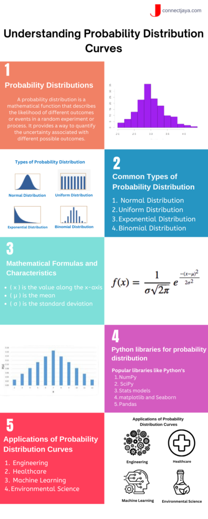
Probability distributions describe the likelihood of various outcomes in a random experiment. They provide a way to visualize and quantify the uncertainty associated with different events. Probability distribution curves, often represented as graphs, illustrate the probability of different outcomes along an axis.

Common Types of Probability Distribution Curves

Several types of probability distribution curves are used to model different scenarios. Let’s explore a few of the most common ones:

Normal Distribution (Gaussian Distribution)

The normal distribution is characterized by its bell-shaped curve and is prevalent in various natural phenomena. It’s parameterized by mean (μ) and standard deviation (σ).

Uniform Distribution:

The uniform distribution represents outcomes with equal probability within a given range. It’s often depicted as a flat, constant curve.

Exponential Distribution

The exponential distribution models the time between events in a Poisson process. It’s commonly used for modeling waiting times.

Binomial Distribution

The binomial distribution describes the number of successes in a fixed number of independent Bernoulli trials. It’s characterized by parameters n (number of trials) and p (probability of success).

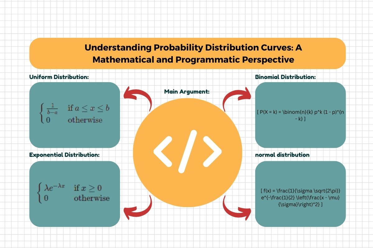
Mathematical Formulas and Characteristics

Each distribution has its own mathematical formula and unique characteristics. For instance, the normal distribution is defined by the probability density function (PDF):

$$[ f(x) = \frac{1}{\sigma \sqrt{2\pi}} e^{-\frac{1}{2} \left(\frac{x – \mu}{\sigma}\right)^2} ]$$

Where:

• ( x ) is the value along the x-axis
• ( \mu ) is the mean
• ( \sigma ) is the standard deviation

Uniform Distribution

The probability density function (PDF) of a uniform distribution is a constant value within a specified interval [a, b], and zero outside that interval:

$$[ f(x) = \begin{cases} \frac{1}{b – a} & \text{if } a \leq x \leq b \\ 0 & \text{otherwise} \end{cases} ]]$$

Exponential Distribution

The PDF of the exponential distribution is often used to model the time between events in a Poisson process. It’s characterized by the parameter (\lambda) (lambda), which is the rate of the process:

$$[ f(x) = \begin{cases} \lambda e^{-\lambda x} & \text{if } x \geq 0 \\ 0 & \text{otherwise} \end{cases}\ ]$$

Binomial Distribution

The probability mass function (PMF) of the binomial distribution represents the probability of having exactly (k) successes in (n) independent Bernoulli trials with probability (p) of success:

$$[ P(X = k) = binom{n}{k} p^k (1 – p)^{n – k} ]$$

Where (\binom{n}{k}) represents the binomial coefficient, given by $$(\frac{n!}{k!(n – k)!}).$$

Programming Probability Distribution Curves

Python and Libraries

Python is a popular language for statistical analysis and visualization. Libraries like NumPy and Matplotlib make it easy to work with probability distributions.

Creating Probability Distributions

 Using NumPy, you can create arrays of random numbers that follow specific probability distributions. For example, to create an array of samples from a normal distribution:

import numpy as np

mean = 0
std_dev = 1
num_samples = 1000

samples = np.random.normal(mean, std_dev, num_samples)

Visualizing Probability Distribution Curves

Matplotlib allows you to visualize probability distribution curves. For a normal distribution

import matplotlib.pyplot as plt
import seaborn as sns

sns.set(style="whitegrid")

plt.figure(figsize=(8, 6))
sns.histplot(samples, kde=True)
plt.title("Normal Distribution")
plt.xlabel("Value")
plt.ylabel("Frequency")
plt.show()

Customizing Plots

Matplotlib offers extensive customization options. You can add labels, legends, and titles, and adjust colors to create informative and visually appealing plots.

plt.figure(figsize=(8, 6))
sns.histplot(samples, kde=True, color='blue', label='Sample Data')
plt.axvline(x=mean, color='red', linestyle='--', label='Mean')
plt.title("Customized Normal Distribution Plot")
plt.xlabel("Value")
plt.ylabel("Frequency")
plt.legend()
plt.show()

Applications of Probability Distribution Curves

Probability distribution curves have extensive applications across various fields:

• Finance: Modeling stock price movements using distributions like the log-normal distribution.
• Physics: Describing particle energies or thermal fluctuations using the Maxwell-Boltzmann distribution.
• Economics: Modeling income distribution using various distributions like Pareto.
• Biology: Analyzing genetics and heredity using the binomial distribution.
• Engineering: In reliability engineering, probability distribution curves help assess the failure rates of components, aiding in designing reliable systems.
• Healthcare: Modeling disease spread and understanding medical test accuracy using distributions like the binomial and normal distributions.
• Machine Learning: In anomaly detection, probability distribution curves help identify data points that deviate significantly from the expected distribution.
• Environmental Science: Analyzing environmental variables like rainfall patterns using various distributions to make predictions.

Conclusion

Probability distribution curves are not only theoretical concepts but practical tools that drive decision-making in diverse fields. Understanding their mathematical foundations and programming implementations empowers professionals and researchers to extract valuable insights from data and make informed choices. As you delve deeper into the realm of probability distribution curves, you’ll find endless opportunities to apply these principles to real-world scenarios, enriching your understanding of uncertainty and randomness. Whether you’re simulating complex systems or analyzing data trends, probability distribution curves stand as essential instruments for interpreting the world around us.