How To Start With Deep Learning using TensorFlow

Step:1 Setup Your Anaconda Environment using VSCode

Step:2 Now we will start working with FASHION-MNIST Dataset

Fashion-MNIST is a dataset of Zalando’s article images consisting of a training set of 60,000 examples and a test set of 10,000 examples. Each example is a 28×28 grayscale image, associated with a label from 10 classes. They intend Fashion-MNIST to serve as a direct drop-in replacement for the original MNIST dataset for benchmarking machine learning algorithms. It shares the same image size and structure of training and testing splits.

Reason Behind Fashion-MNIST

The original MNIST dataset contains a lot of handwritten digits. Members of the AI/ML/Data Science community love this dataset and use it as a benchmark to validate their algorithms. In fact, MNIST is often the first dataset researchers try. There is a saying:

“If it doesn’t work on MNIST, it won’t work at all”, they said. “Well, if it does work on MNIST, it may still fail on others.”

MNIST handwritten Vs MNIST FASHION Side by Side

Source: http://fashion-mnist.s3-website.eu-central-1.amazonaws.com/

Deep Learning : Feed Forward Neural Network Development

# TensorFlow and tf.keras
import tensorflow as tf

# Helper libraries
import numpy as np
import matplotlib.pyplot as plt

print(tf.__version__)


Output:- 2.6.0

Import the Fashion MNIST dataset

This guide uses the Fashion MNIST dataset which contains 70,000 grayscale images in 10 categories. The images show individual articles of clothing at low resolution (28 by 28 pixels), as seen here:

Source: https://github.com/zalandoresearch/fashion-mnist

Fashion MNIST is intended as a drop-in replacement for the classic MNIST dataset—often used as the “Hello, World” of machine learning programs for computer vision. The MNIST dataset contains images of handwritten digits (0, 1, 2, etc.) in a format identical to that of the articles of clothing you’ll use here.

This guide uses Fashion MNIST for variety, and because it’s a slightly more challenging problem than regular MNIST. Both datasets are relatively small and are used to verify that an algorithm works as expected. They’re good starting points to test and debug code.

fashion_mnist = tf.keras.datasets.fashion_mnist

(train_images, train_labels),(test_images, test_labels) = fashion_mnist.load_data()
print(len(train_images))


Output:-
Downloading data from https://storage.googleapis.com/tensorflow/tf-keras-datasets/train-labels-idx1-ubyte.gz
32768/29515 [=================================] - 0s 0us/step
40960/29515 [=========================================] - 0s 0us/step
Downloading data from https://storage.googleapis.com/tensorflow/tf-keras-datasets/train-images-idx3-ubyte.gz
26427392/26421880 [==============================] - 0s 0us/step
26435584/26421880 [==============================] - 0s 0us/step
Downloading data from https://storage.googleapis.com/tensorflow/tf-keras-datasets/t10k-labels-idx1-ubyte.gz
16384/5148 [===============================================================================================] - 0s 0us/step
Downloading data from https://storage.googleapis.com/tensorflow/tf-keras-datasets/t10k-images-idx3-ubyte.gz
4423680/4422102 [==============================] - 0s 0us/step
4431872/4422102 [==============================] - 0s 0us/step
60000

Loading the dataset returns four NumPy arrays:

The train_images and train_labels arrays are the training set—the data the model uses to learn.
The model is tested against the test set, the test_images, and test_labels arrays.

The images are 28×28 NumPy arrays, with pixel values ranging from 0 to 255. The labels are an array of integers, ranging from 0 to 9. These correspond to the class of clothing the image represents:

Label	Class
0	T-shirt/top
1	Trouser
2	Pullover
3	Dress
4	Coat
5	Sandal
6	Shirt
7	Sneaker
8	Bag
9	Ankle boot

Each image is mapped to a single label. Since the class names are not included with the dataset, store them here to use later when plotting the images:

class_names = ['T-shirt/top', 'Trouser', 'Pullover', 'Dress', 'Coat','Sandal', 'Shirt', 'Sneaker', 'Bag', 'Ankle boot']
print(class_names)


Output:-  ['T-shirt/top',
 'Trouser',
 'Pullover',
 'Dress',
 'Coat',
 'Sandal',
 'Shirt',
 'Sneaker',
 'Bag',
 'Ankle boot']

Explore the data

Let’s explore the format of the dataset before training the model. The following shows there are 60,000 images in the training set, with each image represented as 28 x 28 pixels:

train_images.shape


Output:-  (60000, 28, 28)

Likewise, there are 60,000 labels in the training set:

len(train_labels)


Output:- 60000

Each label is an integer between 0 and 9:

train_labels


Output:-  array([9, 0, 0, ..., 3, 0, 5], dtype=uint8)

There are 10,000 images in the test set. Again, each image is represented as 28 x 28 pixels:

test_images.shape

Output:-  
(10000, 28, 28)

And the test set contains 10,000 images labels:

len(test_labels)

Output:-  10000

Preprocess the data

The data must be preprocessed before training the network. If you inspect the first image in the training set, you will see that the pixel values fall in the range of 0 to 255:

plt.figure()
plt.imshow(train_images[1])
plt.colorbar()
plt.grid(True)
plt.show()


Output:-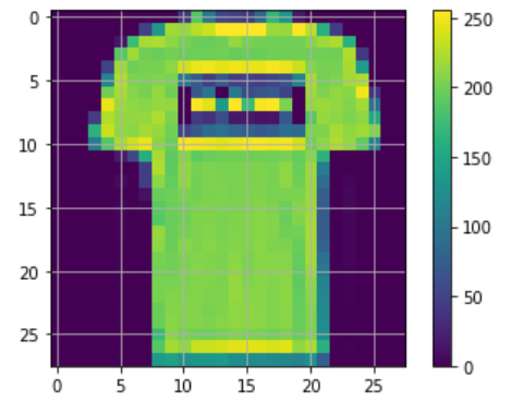

Scale these values to a range of 0 to 1 before feeding them to the neural network model. To do so, divide the values by 255. It’s important that the training set and the testing set be preprocessed in the same way:

train_images = train_images / 255.0

test_images = test_images / 255.0

To verify that the data is in the correct format and that you’re ready to build and train the network, let’s display the first 25 images from the training set and display the class name below each image.

plt.figure(figsize=(5,5))
for i in range(25):
    plt.subplot(5,5,1+i)
    plt.xticks([])
    plt.yticks([])
    plt.grid(False)
    plt.imshow(train_images[i], cmap=plt.cm.binary)
    plt.xlabel(class_names[train_labels[i]])
plt.show()


Output:-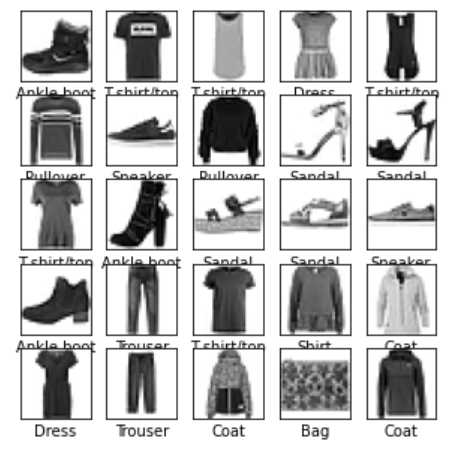

Build the model

Building the neural network requires configuring the layers of the model, then compiling the model.

Set up the layers

The basic building block of a neural network is the layer. Layers extract representations from the data fed into them. Hopefully, these representations are meaningful for the problem at hand.

Most of deep learning consists of chaining together simple layers. Most layers, such as tf.keras.layers.Dense, have parameters that are learned during training.

model = tf.keras.Sequential([
    tf.keras.layers.Flatten(input_shape=(28, 28)),
    tf.keras.layers.Dense(128, activation='relu'),
    tf.keras.layers.Dense(10)
])

model.summary()


Output:-
Model: "sequential"
_________________________________________________________________
Layer (type)                 Output Shape              Param #   
=================================================================
flatten (Flatten)            (None, 784)               0         
_________________________________________________________________
dense (Dense)                (None, 128)               100480    
_________________________________________________________________
dense_1 (Dense)              (None, 10)                1290      
=================================================================
Total params: 101,770
Trainable params: 101,770
Non-trainable params: 0
_________________________________________________________________

The first layer in this network, tf.keras.layers.Flatten, transforms the format of the images from a two-dimensional array (of 28 by 28 pixels) to a one-dimensional array (of 28 * 28 = 784 pixels). Think of this layer as unstacking rows of pixels in the image and lining them up. This layer has no parameters to learn; it only reformats the data.

After the pixels are flattened, the network consists of a sequence of two tf.keras.layers.Dense layers. These are densely connected, or fully connected, neural layers. The first Dense layer has 128 nodes (or neurons). The second (and last) layer returns a logits array with length of 10. Each node contains a score that indicates the current image belongs to one of the 10 classes.

Compile the model

Before the model is ready for training, it needs a few more settings. These are added during the model’s compile step:

Loss function —This measures how accurate the model is during training. You want to minimize this function to “steer” the model in the right direction.
Optimizer —This is how the model is updated based on the data it sees and its loss function.
Metrics —Used to monitor the training and testing steps. The following example uses accuracy, the fraction of the images that are correctly classified.

model.compile(optimizer='adam',
              loss=tf.keras.losses.SparseCategoricalCrossentropy(from_logits=True),
              metrics=['accuracy'])

Train the model

Training the neural network model requires the following steps:

Feed the training data to the model. In this example, the training data is in the train_images and train_labels arrays.
The model learns to associate images and labels.
You ask the model to make predictions about a test set—in this example, the test_images array.
Verify that the predictions match the labels from the test_labels array.

Feed the model

To start training, call the model.fit method—so called because it “fits” the model to the training data:

model.fit(train_images, train_labels, epochs=10)


Output:-
Epoch 1/10
1875/1875 [==============================] - 4s 2ms/step - loss: 1.1166 - accuracy: 0.6635
Epoch 2/10
1875/1875 [==============================] - 4s 2ms/step - loss: 0.6536 - accuracy: 0.7642
Epoch 3/10
1875/1875 [==============================] - 4s 2ms/step - loss: 0.5762 - accuracy: 0.7936
Epoch 4/10
1875/1875 [==============================] - 4s 2ms/step - loss: 0.5316 - accuracy: 0.8114
Epoch 5/10
1875/1875 [==============================] - 4s 2ms/step - loss: 0.5019 - accuracy: 0.8221
Epoch 6/10
1875/1875 [==============================] - 4s 2ms/step - loss: 0.4802 - accuracy: 0.8297
Epoch 7/10
1875/1875 [==============================] - 4s 2ms/step - loss: 0.4637 - accuracy: 0.8366
Epoch 8/10
1875/1875 [==============================] - 4s 2ms/step - loss: 0.4511 - accuracy: 0.8408
Epoch 9/10
1875/1875 [==============================] - 4s 2ms/step - loss: 0.4406 - accuracy: 0.8431
Epoch 10/10
1875/1875 [==============================] - 4s 2ms/step - loss: 0.4318 - accuracy: 0.8474
<keras.callbacks.History at 0x7f286ee78250>

As the model trains, the loss and accuracy metrics are displayed. This model reaches an accuracy of about 0.91 (or 91%) on the training data.

Evaluate accuracy

Next, compare how the model performs on the test dataset:

test_loss, test_acc = model.evaluate(test_images,  test_labels, verbose=2)

print('\nTest accuracy:', test_acc)


Output:-
313/313 - 0s - loss: 0.4583 - accuracy: 0.8342

Test accuracy: 0.8342000246047974

It turns out that the accuracy on the test dataset is a little less than the accuracy on the training dataset. This gap between training accuracy and test accuracy represents overfitting. Overfitting happens when a machine learning model performs worse on new, previously unseen inputs than it does on the training data. An overfitted model “memorizes” the noise and details in the training dataset to a point where it negatively impacts the performance of the model on the new data. For more information, see the following:

Make predictions

With the model trained, you can use it to make predictions about some images. The model’s linear outputs, logits. Attach a softmax layer to convert the logits to probabilities, which are easier to interpret.

probability_model = tf.keras.Sequential([model, 
                                         tf.keras.layers.Softmax()])

predictions = probability_model.predict(test_images)

Here, the model has predicted the label for each image in the testing set. Let’s take a look at the first prediction:

predictions[0]


Output:-array([5.6716897e-07, 4.2498094e-08, 4.3915343e-06, 6.5611953e-06,
       8.6530908e-06, 1.2003078e-01, 8.9145060e-06, 3.2775763e-01,
       6.0194274e-03, 5.4616308e-01], dtype=float32)

A prediction is an array of 10 numbers. They represent the model’s “confidence” that the image corresponds to each of the 10 different articles of clothing. You can see which label has the highest confidence value:

np.argmax(predictions[1]) 

Output:- 2

So, the model is most confident that this image is an ankle boot, or class_names[9]. Examining the test label shows that this classification is correct:

test_labels[1]


Output:-

Graph this to look at the full set of 10 class predictions.

def plot_image(i, predictions_array, true_label, img):
  true_label, img = true_label[i], img[i]
  plt.grid(False)
  plt.xticks([])
  plt.yticks([])

  plt.imshow(img, cmap=plt.cm.binary)

  predicted_label = np.argmax(predictions_array)
  if predicted_label == true_label:
    color = 'blue'
  else:
    color = 'red'

  plt.xlabel("{} {:2.0f}% ({})".format(class_names[predicted_label],
                                100*np.max(predictions_array),
                                class_names[true_label]),
                                color=color)

def plot_value_array(i, predictions_array, true_label):
  true_label = true_label[i]
  plt.grid(False)
  plt.xticks(range(10))
  plt.yticks([])
  thisplot = plt.bar(range(10), predictions_array, color="#777777")
  plt.ylim([0, 1])
  predicted_label = np.argmax(predictions_array)

  thisplot[predicted_label].set_color('red')
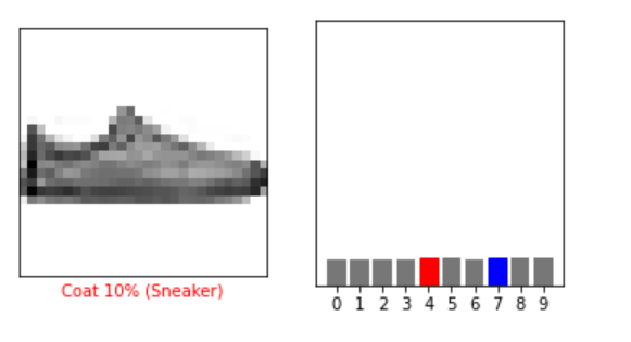
  thisplot[true_label].set_color('blue')

Verify predictions

With the model trained, you can use it to make predictions about some images.

Let’s look at the 0th image, predictions, and prediction array. Correct prediction labels are blue and incorrect prediction labels are red. The number gives the percentage (out of 100) for the predicted label.

i = 1
plt.figure(figsize=(6,3))
plt.subplot(1,2,1)
plot_image(i, predictions[i], test_labels, test_images)
plt.subplot(1,2,2)
plot_value_array(i, predictions[i],  test_labels)
plt.show()


Output:-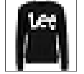

i = 12
plt.figure(figsize=(6,3))
plt.subplot(1,2,1)
plot_image(i, predictions[i], test_labels, test_images)
plt.subplot(1,2,2)
plot_value_array(i, predictions[i],  test_labels)
plt.show()


Output:-

Let’s plot several images with their predictions. Note that the model can be wrong even when very confident.CodeText

# Plot the first X test images, their predicted labels, and the true labels.
# Color correct predictions in blue and incorrect predictions in red.
num_rows = 5
num_cols = 3
num_images = num_rows*num_cols
plt.figure(figsize=(2*2*num_cols, 2*num_rows))
for i in range(num_images):
  plt.subplot(num_rows, 2*num_cols, 2*i+1)
  plot_image(i, predictions[i], test_labels, test_images)
  plt.subplot(num_rows, 2*num_cols, 2*i+2)
  plot_value_array(i, predictions[i], test_labels)
plt.tight_layout()
plt.show()

Use the trained model

Finally, use the trained model to make a prediction about a single image.

# Grab an image from the test dataset.
img = test_images[1]

print(img.shape)


Output:- (28, 28)

tf.keras models are optimized to make predictions on a batch, or collection, of examples at once. Accordingly, even though you’re using a single image, you need to add it to a list:

# Add the image to a batch where it's the only member.
img = (np.expand_dims(img,0))

print(img.shape)


Output:-  (1, 28, 28)

Now predict the correct label for this image:

predictions_single = probability_model.predict(img)

print(predictions_single)


Output:-
[[1.9217783e-04 3.3568033e-06 9.0862662e-01 4.0786781e-05 1.3652470e-02
  1.7151864e-09 7.7396996e-02 3.3897265e-15 8.7664383e-05 4.1771864e-12]]

plot_value_array(1, predictions_single[0], test_labels)
_ = plt.xticks(range(10), class_names, rotation=45)
plt.show()


Output:-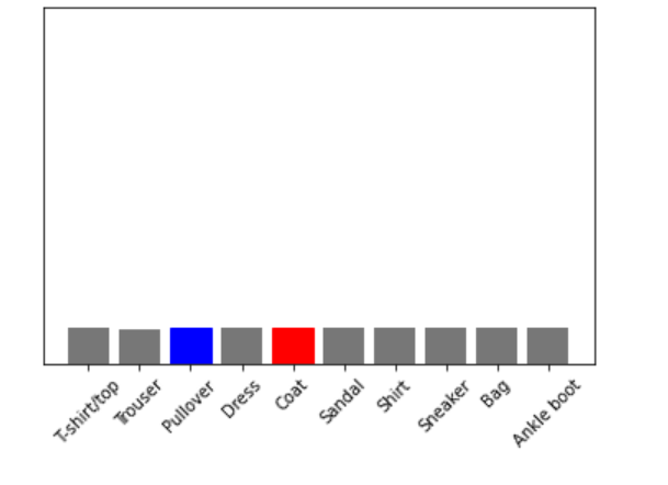

tf.keras.Model.predict returns a list of lists—one list for each image in the batch of data. Grab the predictions for our (only) image in the batch:CodeText

np.argmax(predictions_single[0])


Output:- 2

And the model predicts a label as expected.

Tech insights for the curious mind