
Nearly all scientific fields have felt the impact of this technology. Most industries and businesses have already been disrupted and transformed through the use of DL. The leading technology and economy-focused companies around the world are in a race to improve DL. Even now, human-level performance and capability cannot exceed that of the performance of DL in many areas, such as predicting the time taken to make car deliveries, decisions to certify loan requests, and predicting movie ratings
DL has become the main tool in many hospitals around the world for automatic COVID-19 classification and detection using chest X-ray images or other types of images. We end this section by the saying of AI pioneer Geoffrey Hinton
“Deep learning is going to be able to do everything”.
Geoffrey Hinton
When to apply deep learning?
Machine intelligence is useful in many situations which is equal or better than human experts in some cases, meaning that DL can be a solution to the following problems:
- Cases where human experts are not available.
- Cases where humans are unable to explain decisions made using their expertise (language understanding, medical decisions, and speech recognition).
- Cases where the problem solution updates over time (price prediction, stock preference, weather prediction, and tracking).
- Cases where solutions require adaptation based on specific cases (personalization, biometrics).
- Cases where the size of the problem is extremely large and exceeds our inadequate reasoning abilities (sentiment analysis, matching ads to Facebook, calculation webpage ranks).
Why deep learning?
Several performance features may answer this question, e.g
- Universal Learning Approach: Because DL has the ability to perform in approximately all application domains, it is sometimes referred to as universal learning.
- Robustness: In general, precisely designed features are not required in DL techniques. Instead, the optimized features are learned in an automated fashion related to the task under consideration. Thus, robustness to the usual changes of the input data is attained.
- Generalization: Different data types or different applications can use the same DL technique, an approach frequently referred to as transfer learning (TL) which explained in the latter section. Furthermore, it is a useful approach in problems where data is insufficient.
- Scalability: DL is highly scalable. ResNet, which was invented by Microsoft, comprises 1202 layers and is frequently applied at a supercomputing scale. Lawrence Livermore National Laboratory (LLNL), a large enterprise working on evolving frameworks for networks, adopted a similar approach, where thousands of nodes can be implemented.
The most famous types of deep learning networks are discussed in this section are CNNs.
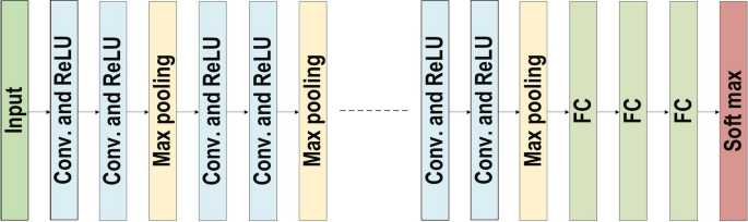
Convolutional Neural Networks (CNNs)
The main benefit of CNN compared to its predecessors is that it automatically identifies the relevant features without any human supervision.
Benefits of employing CNNs
The benefits of using CNNs over other traditional neural networks in the computer vision environment are listed as follows:
- The main reason to consider CNN is the weight-sharing feature, which reduces the number of trainable network parameters and in turn helps the network to enhance generalization and avoid over-fitting.
- Concurrently learning the feature extraction layers and the classification layer causes the model output to be both highly organized and highly reliant on the extracted features.
- Large-scale network implementation is much easier with CNN than with other neural networks.
CNN Architectures
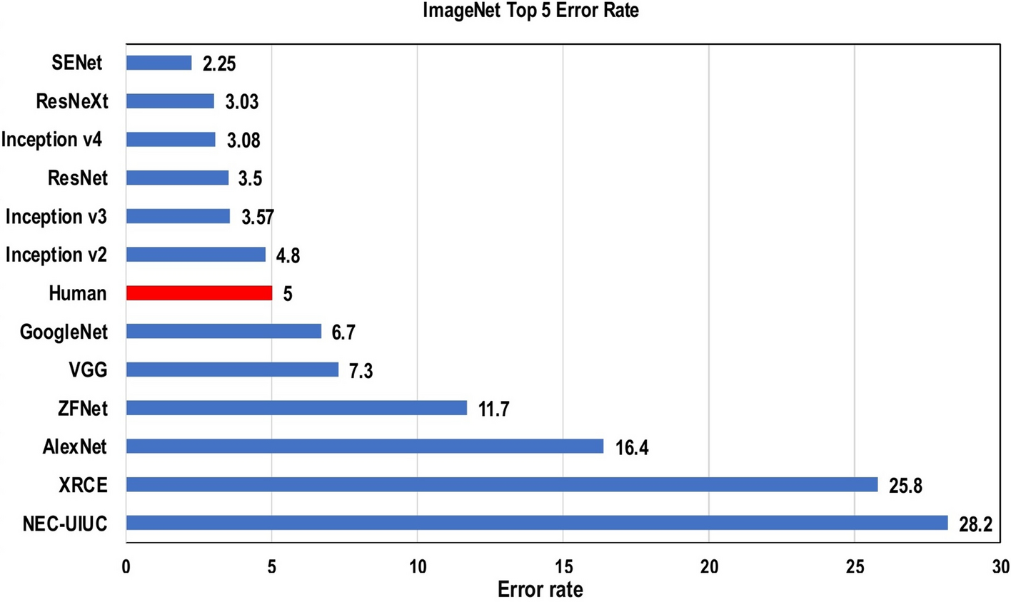
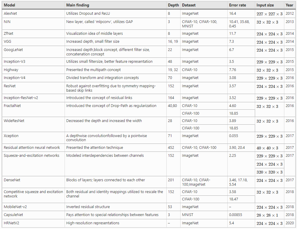
Over the last 10 years, several CNN architectures have been presented. Model architecture is a critical factor in improving the performance of different applications. Various modifications have been achieved in CNN architecture from 1989 until today. Such modifications include structural reformulation, regularization, parameter optimizations, etc. Conversely, it should be noted that the key upgrade in CNN performance occurred largely due to the processing-unit reorganization, as well as the development of novel blocks. In particular, the most novel developments in CNN architectures were performed on the use of network depth. In this section, we review the most popular CNN architectures, beginning from the AlexNet model in 2012 and ending at the High-Resolution (HR) model in 2020.
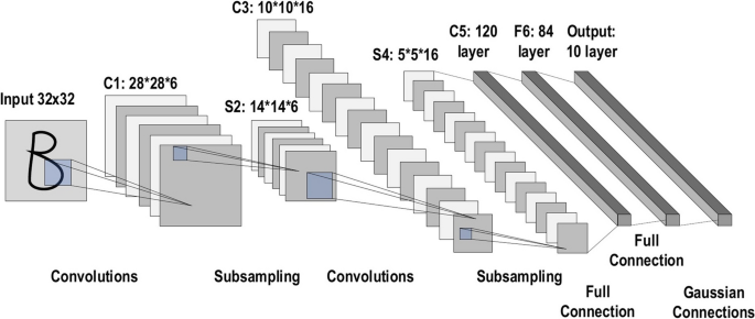
LeNet
The history of deep CNNs began with the appearance of LeNet. At that time, the CNNs were restricted to handwritten digit recognition tasks, which cannot be scaled to all image classes.
AlexNet
In deep CNN architecture, AlexNet is highly respected, as it achieved innovative results in the fields of image recognition and classification. Krizhevesky et al. first proposed AlexNet and consequently improved the CNN learning ability by increasing its depth and implementing several parameter optimization strategies.
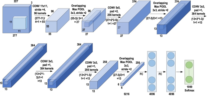
The learning ability of the deep CNN was limited at this time due to hardware restrictions. To overcome these hardware limitations, two GPUs (NVIDIA GTX 580) were used in parallel to train AlexNet. Moreover, in order to enhance the applicability of the CNN to different image categories, the number of feature extraction stages was increased from five in LeNet to seven in AlexNet.
Visual geometry group (VGG)
After CNN was determined to be effective in the field of image recognition, an easy and efficient design principle for CNN was proposed by Simonyan and Zisserman. This innovative design was called Visual Geometry Group (VGG).
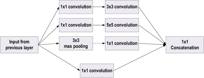
GoogLeNet
In the 2014-ILSVRC competition, GoogleNet (also called Inception-V1) emerged as the winner. Achieving high-level accuracy with decreased computational cost is the core aim of the GoogleNet architecture. It proposed a novel inception block (module) concept in the CNN context, since it combines multiple-scale convolutional transformations by employing merge, transform, and split functions for feature extraction.
The motivation of GoogLeNet was to improve the efficiency of CNN parameters, as well as to enhance the learning capacity. In addition, it regulates the computation by inserting a 1×1 convolutional filter, as a bottleneck layer, ahead of using large-size kernels.
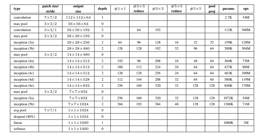
GoogLeNet model Summary
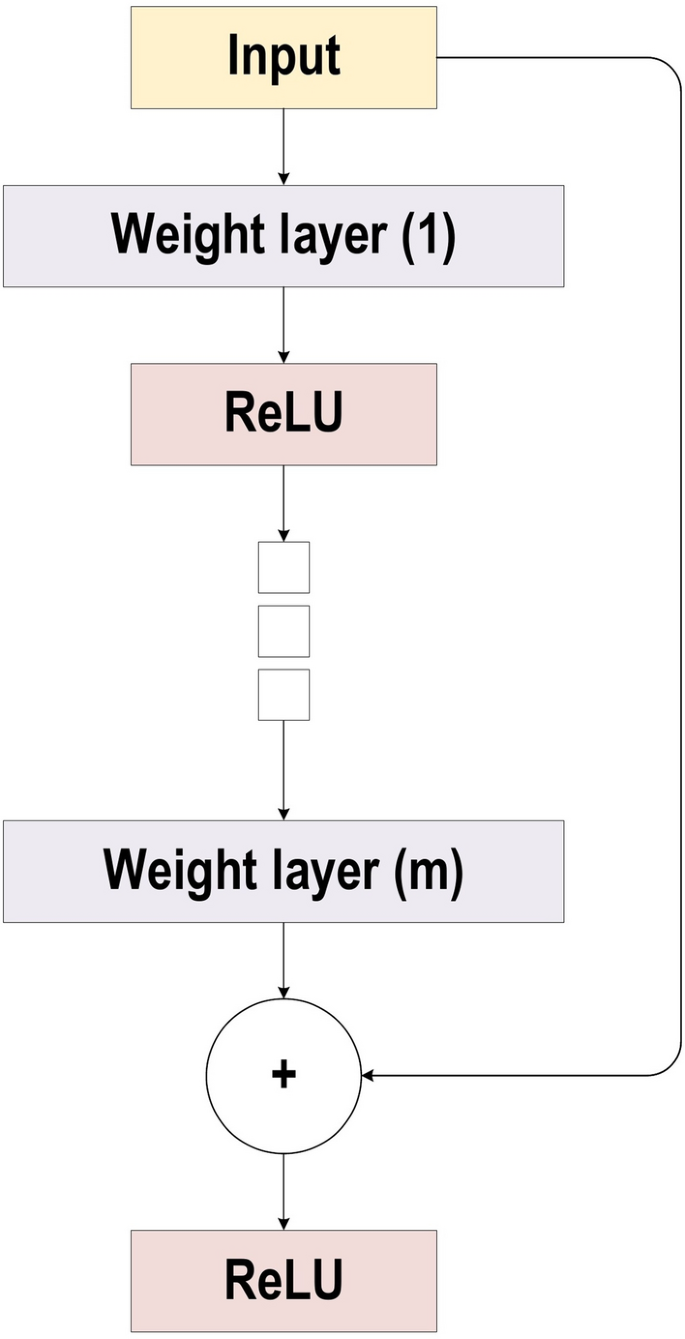
ResNet
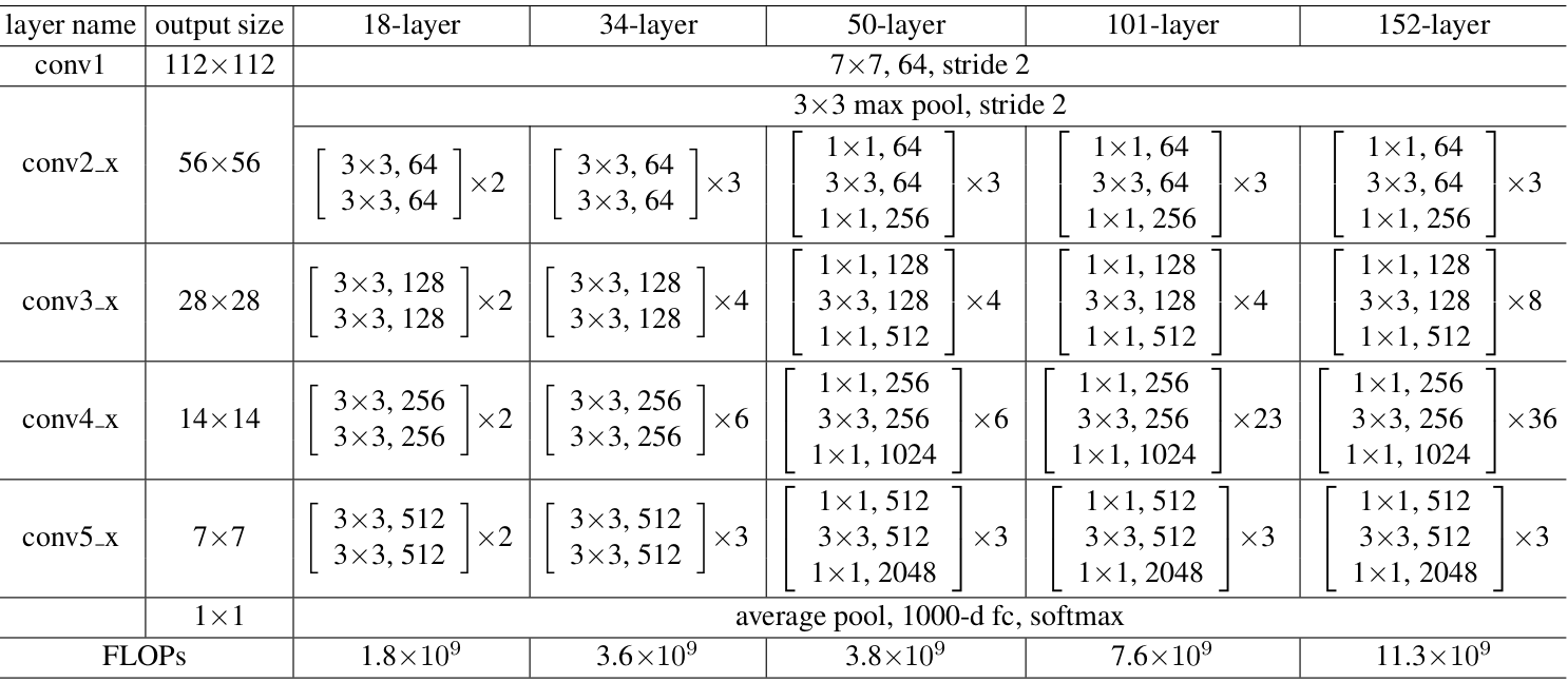
He et al. developed ResNet (Residual Network), which was the winner of ILSVRC 2015. Their objective was to design an ultra-deep network free of the vanishing gradient issue, as compared to the previous networks. Several types of ResNet were developed based on the number of layers (starting with 34 layers and going up to 1202 layers). The most common type was ResNet50, which comprised 49 convolutional layers plus a single FC layer. The overall number of network weights was 25.5 M, while the overall number of MACs was 3.9 M. The novel idea of ResNet is its use of the bypass pathway concept.
ResNet has the potential to prevent the problems of gradient diminishing, as the shortcut connections (residual links) accelerate the deep network convergence. ResNet was the winner of the 2015-ILSVRC championship with 152 layers of depth; this represents 8 times the depth of VGG and 20 times the depth of AlexNet. In comparison with VGG, it has lower computational complexity, even with enlarged depth.
Resnet Model summary
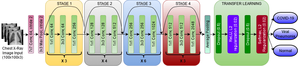
ResNet50 Model Summary:
model = models.resnet50(pretrained=True)Output:
ResNet(
  (conv1): Conv2d(3, 64, kernel_size=(7, 7), stride=(2, 2), padding=(3, 3), bias=False)
  (bn1): BatchNorm2d(64, eps=1e-05, momentum=0.1, affine=True, track_running_stats=True)
  (relu): ReLU(inplace=True)
  (maxpool): MaxPool2d(kernel_size=3, stride=2, padding=1, dilation=1, ceil_mode=False)
  (layer1): Sequential(
    (0): Bottleneck(
      (conv1): Conv2d(64, 64, kernel_size=(1, 1), stride=(1, 1), bias=False)
      (bn1): BatchNorm2d(64, eps=1e-05, momentum=0.1, affine=True, track_running_stats=True)
      (conv2): Conv2d(64, 64, kernel_size=(3, 3), stride=(1, 1), padding=(1, 1), bias=False)
      (bn2): BatchNorm2d(64, eps=1e-05, momentum=0.1, affine=True, track_running_stats=True)
      (conv3): Conv2d(64, 256, kernel_size=(1, 1), stride=(1, 1), bias=False)
      (bn3): BatchNorm2d(256, eps=1e-05, momentum=0.1, affine=True, track_running_stats=True)
      (relu): ReLU(inplace=True)
      (downsample): Sequential(
        (0): Conv2d(64, 256, kernel_size=(1, 1), stride=(1, 1), bias=False)
        (1): BatchNorm2d(256, eps=1e-05, momentum=0.1, affine=True, track_running_stats=True)
      )
    )
    (1): Bottleneck(
      (conv1): Conv2d(256, 64, kernel_size=(1, 1), stride=(1, 1), bias=False)
      (bn1): BatchNorm2d(64, eps=1e-05, momentum=0.1, affine=True, track_running_stats=True)
      (conv2): Conv2d(64, 64, kernel_size=(3, 3), stride=(1, 1), padding=(1, 1), bias=False)
      (bn2): BatchNorm2d(64, eps=1e-05, momentum=0.1, affine=True, track_running_stats=True)
      (conv3): Conv2d(64, 256, kernel_size=(1, 1), stride=(1, 1), bias=False)
      (bn3): BatchNorm2d(256, eps=1e-05, momentum=0.1, affine=True, track_running_stats=True)
      (relu): ReLU(inplace=True)
    )
    (2): Bottleneck(
      (conv1): Conv2d(256, 64, kernel_size=(1, 1), stride=(1, 1), bias=False)
      (bn1): BatchNorm2d(64, eps=1e-05, momentum=0.1, affine=True, track_running_stats=True)
      (conv2): Conv2d(64, 64, kernel_size=(3, 3), stride=(1, 1), padding=(1, 1), bias=False)
      (bn2): BatchNorm2d(64, eps=1e-05, momentum=0.1, affine=True, track_running_stats=True)
      (conv3): Conv2d(64, 256, kernel_size=(1, 1), stride=(1, 1), bias=False)
      (bn3): BatchNorm2d(256, eps=1e-05, momentum=0.1, affine=True, track_running_stats=True)
      (relu): ReLU(inplace=True)
    )
  )
  (layer2): Sequential(
    (0): Bottleneck(
      (conv1): Conv2d(256, 128, kernel_size=(1, 1), stride=(1, 1), bias=False)
      (bn1): BatchNorm2d(128, eps=1e-05, momentum=0.1, affine=True, track_running_stats=True)
      (conv2): Conv2d(128, 128, kernel_size=(3, 3), stride=(2, 2), padding=(1, 1), bias=False)
      (bn2): BatchNorm2d(128, eps=1e-05, momentum=0.1, affine=True, track_running_stats=True)
      (conv3): Conv2d(128, 512, kernel_size=(1, 1), stride=(1, 1), bias=False)
      (bn3): BatchNorm2d(512, eps=1e-05, momentum=0.1, affine=True, track_running_stats=True)
      (relu): ReLU(inplace=True)
      (downsample): Sequential(
        (0): Conv2d(256, 512, kernel_size=(1, 1), stride=(2, 2), bias=False)
        (1): BatchNorm2d(512, eps=1e-05, momentum=0.1, affine=True, track_running_stats=True)
      )
    )
    (1): Bottleneck(
      (conv1): Conv2d(512, 128, kernel_size=(1, 1), stride=(1, 1), bias=False)
      (bn1): BatchNorm2d(128, eps=1e-05, momentum=0.1, affine=True, track_running_stats=True)
      (conv2): Conv2d(128, 128, kernel_size=(3, 3), stride=(1, 1), padding=(1, 1), bias=False)
      (bn2): BatchNorm2d(128, eps=1e-05, momentum=0.1, affine=True, track_running_stats=True)
      (conv3): Conv2d(128, 512, kernel_size=(1, 1), stride=(1, 1), bias=False)
      (bn3): BatchNorm2d(512, eps=1e-05, momentum=0.1, affine=True, track_running_stats=True)
      (relu): ReLU(inplace=True)
    )
    (2): Bottleneck(
      (conv1): Conv2d(512, 128, kernel_size=(1, 1), stride=(1, 1), bias=False)
      (bn1): BatchNorm2d(128, eps=1e-05, momentum=0.1, affine=True, track_running_stats=True)
      (conv2): Conv2d(128, 128, kernel_size=(3, 3), stride=(1, 1), padding=(1, 1), bias=False)
      (bn2): BatchNorm2d(128, eps=1e-05, momentum=0.1, affine=True, track_running_stats=True)
      (conv3): Conv2d(128, 512, kernel_size=(1, 1), stride=(1, 1), bias=False)
      (bn3): BatchNorm2d(512, eps=1e-05, momentum=0.1, affine=True, track_running_stats=True)
      (relu): ReLU(inplace=True)
    )
    (3): Bottleneck(
      (conv1): Conv2d(512, 128, kernel_size=(1, 1), stride=(1, 1), bias=False)
      (bn1): BatchNorm2d(128, eps=1e-05, momentum=0.1, affine=True, track_running_stats=True)
      (conv2): Conv2d(128, 128, kernel_size=(3, 3), stride=(1, 1), padding=(1, 1), bias=False)
      (bn2): BatchNorm2d(128, eps=1e-05, momentum=0.1, affine=True, track_running_stats=True)
      (conv3): Conv2d(128, 512, kernel_size=(1, 1), stride=(1, 1), bias=False)
      (bn3): BatchNorm2d(512, eps=1e-05, momentum=0.1, affine=True, track_running_stats=True)
      (relu): ReLU(inplace=True)
    )
  )
  (layer3): Sequential(
    (0): Bottleneck(
      (conv1): Conv2d(512, 256, kernel_size=(1, 1), stride=(1, 1), bias=False)
      (bn1): BatchNorm2d(256, eps=1e-05, momentum=0.1, affine=True, track_running_stats=True)
      (conv2): Conv2d(256, 256, kernel_size=(3, 3), stride=(2, 2), padding=(1, 1), bias=False)
      (bn2): BatchNorm2d(256, eps=1e-05, momentum=0.1, affine=True, track_running_stats=True)
      (conv3): Conv2d(256, 1024, kernel_size=(1, 1), stride=(1, 1), bias=False)
      (bn3): BatchNorm2d(1024, eps=1e-05, momentum=0.1, affine=True, track_running_stats=True)
      (relu): ReLU(inplace=True)
      (downsample): Sequential(
        (0): Conv2d(512, 1024, kernel_size=(1, 1), stride=(2, 2), bias=False)
        (1): BatchNorm2d(1024, eps=1e-05, momentum=0.1, affine=True, track_running_stats=True)
      )
    )
    (1): Bottleneck(
      (conv1): Conv2d(1024, 256, kernel_size=(1, 1), stride=(1, 1), bias=False)
      (bn1): BatchNorm2d(256, eps=1e-05, momentum=0.1, affine=True, track_running_stats=True)
      (conv2): Conv2d(256, 256, kernel_size=(3, 3), stride=(1, 1), padding=(1, 1), bias=False)
      (bn2): BatchNorm2d(256, eps=1e-05, momentum=0.1, affine=True, track_running_stats=True)
      (conv3): Conv2d(256, 1024, kernel_size=(1, 1), stride=(1, 1), bias=False)
      (bn3): BatchNorm2d(1024, eps=1e-05, momentum=0.1, affine=True, track_running_stats=True)
      (relu): ReLU(inplace=True)
    )
    (2): Bottleneck(
      (conv1): Conv2d(1024, 256, kernel_size=(1, 1), stride=(1, 1), bias=False)
      (bn1): BatchNorm2d(256, eps=1e-05, momentum=0.1, affine=True, track_running_stats=True)
      (conv2): Conv2d(256, 256, kernel_size=(3, 3), stride=(1, 1), padding=(1, 1), bias=False)
      (bn2): BatchNorm2d(256, eps=1e-05, momentum=0.1, affine=True, track_running_stats=True)
      (conv3): Conv2d(256, 1024, kernel_size=(1, 1), stride=(1, 1), bias=False)
      (bn3): BatchNorm2d(1024, eps=1e-05, momentum=0.1, affine=True, track_running_stats=True)
      (relu): ReLU(inplace=True)
    )
    (3): Bottleneck(
      (conv1): Conv2d(1024, 256, kernel_size=(1, 1), stride=(1, 1), bias=False)
      (bn1): BatchNorm2d(256, eps=1e-05, momentum=0.1, affine=True, track_running_stats=True)
      (conv2): Conv2d(256, 256, kernel_size=(3, 3), stride=(1, 1), padding=(1, 1), bias=False)
      (bn2): BatchNorm2d(256, eps=1e-05, momentum=0.1, affine=True, track_running_stats=True)
      (conv3): Conv2d(256, 1024, kernel_size=(1, 1), stride=(1, 1), bias=False)
      (bn3): BatchNorm2d(1024, eps=1e-05, momentum=0.1, affine=True, track_running_stats=True)
      (relu): ReLU(inplace=True)
    )
    (4): Bottleneck(
      (conv1): Conv2d(1024, 256, kernel_size=(1, 1), stride=(1, 1), bias=False)
      (bn1): BatchNorm2d(256, eps=1e-05, momentum=0.1, affine=True, track_running_stats=True)
      (conv2): Conv2d(256, 256, kernel_size=(3, 3), stride=(1, 1), padding=(1, 1), bias=False)
      (bn2): BatchNorm2d(256, eps=1e-05, momentum=0.1, affine=True, track_running_stats=True)
      (conv3): Conv2d(256, 1024, kernel_size=(1, 1), stride=(1, 1), bias=False)
      (bn3): BatchNorm2d(1024, eps=1e-05, momentum=0.1, affine=True, track_running_stats=True)
      (relu): ReLU(inplace=True)
    )
    (5): Bottleneck(
      (conv1): Conv2d(1024, 256, kernel_size=(1, 1), stride=(1, 1), bias=False)
      (bn1): BatchNorm2d(256, eps=1e-05, momentum=0.1, affine=True, track_running_stats=True)
      (conv2): Conv2d(256, 256, kernel_size=(3, 3), stride=(1, 1), padding=(1, 1), bias=False)
      (bn2): BatchNorm2d(256, eps=1e-05, momentum=0.1, affine=True, track_running_stats=True)
      (conv3): Conv2d(256, 1024, kernel_size=(1, 1), stride=(1, 1), bias=False)
      (bn3): BatchNorm2d(1024, eps=1e-05, momentum=0.1, affine=True, track_running_stats=True)
      (relu): ReLU(inplace=True)
    )
  )
  (layer4): Sequential(
    (0): Bottleneck(
      (conv1): Conv2d(1024, 512, kernel_size=(1, 1), stride=(1, 1), bias=False)
      (bn1): BatchNorm2d(512, eps=1e-05, momentum=0.1, affine=True, track_running_stats=True)
      (conv2): Conv2d(512, 512, kernel_size=(3, 3), stride=(2, 2), padding=(1, 1), bias=False)
      (bn2): BatchNorm2d(512, eps=1e-05, momentum=0.1, affine=True, track_running_stats=True)
      (conv3): Conv2d(512, 2048, kernel_size=(1, 1), stride=(1, 1), bias=False)
      (bn3): BatchNorm2d(2048, eps=1e-05, momentum=0.1, affine=True, track_running_stats=True)
      (relu): ReLU(inplace=True)
      (downsample): Sequential(
        (0): Conv2d(1024, 2048, kernel_size=(1, 1), stride=(2, 2), bias=False)
        (1): BatchNorm2d(2048, eps=1e-05, momentum=0.1, affine=True, track_running_stats=True)
      )
    )
    (1): Bottleneck(
      (conv1): Conv2d(2048, 512, kernel_size=(1, 1), stride=(1, 1), bias=False)
      (bn1): BatchNorm2d(512, eps=1e-05, momentum=0.1, affine=True, track_running_stats=True)
      (conv2): Conv2d(512, 512, kernel_size=(3, 3), stride=(1, 1), padding=(1, 1), bias=False)
      (bn2): BatchNorm2d(512, eps=1e-05, momentum=0.1, affine=True, track_running_stats=True)
      (conv3): Conv2d(512, 2048, kernel_size=(1, 1), stride=(1, 1), bias=False)
      (bn3): BatchNorm2d(2048, eps=1e-05, momentum=0.1, affine=True, track_running_stats=True)
      (relu): ReLU(inplace=True)
    )
    (2): Bottleneck(
      (conv1): Conv2d(2048, 512, kernel_size=(1, 1), stride=(1, 1), bias=False)
      (bn1): BatchNorm2d(512, eps=1e-05, momentum=0.1, affine=True, track_running_stats=True)
      (conv2): Conv2d(512, 512, kernel_size=(3, 3), stride=(1, 1), padding=(1, 1), bias=False)
      (bn2): BatchNorm2d(512, eps=1e-05, momentum=0.1, affine=True, track_running_stats=True)
      (conv3): Conv2d(512, 2048, kernel_size=(1, 1), stride=(1, 1), bias=False)
      (bn3): BatchNorm2d(2048, eps=1e-05, momentum=0.1, affine=True, track_running_stats=True)
      (relu): ReLU(inplace=True)
    )
  )
  (avgpool): AdaptiveAvgPool2d(output_size=(1, 1))
  (fc): Linear(in_features=2048, out_features=1000, bias=True)
)
ResNet50 Application on COVID Data:
