
Universal Functions: Fast Element-Wise Array Functions
A universal function, or ufunc, is a function that performs element-wise operations on data in ndarrays. You can think of them as fast vectorized wrappers for simple functions that take one or more scalar values and produce one or more scalar results.
Many ufuncs are simple element-wise transformations, like sqrt or exp:
In [1]: arr = np.arange(10)
In [2]: arr
Output: array([0, 1, 2, 3, 4, 5, 6, 7, 8, 9])
In [3]: np.sqrt(arr)
Output: array([0.        , 1.        , 1.41421356, 1.73205081, 2.        ,
               2.23606798, 2.44948974, 2.64575131, 2.82842712, 3.        ])
In[4]: np.exp(arr)
Output: array([1.00000000e+00, 2.71828183e+00, 7.38905610e+00, 2.00855369e+01,
               5.45981500e+01, 1.48413159e+02, 4.03428793e+02, 1.09663316e+03,
               2.98095799e+03, 8.10308393e+03])
These are referred to as unary ufuncs. Others, such as add or maximum, take two arrays (thus, binary ufuncs) and return a single array as the result:
In [5]: x = np.random.randn(8)
In [6]: y = np.random.randn(8)
In [7]: x
Output: array([-0.02290426, -0.08916755,  0.88118988, -0.52292579,  1.13871   ,
                0.67017463,  0.88709011, -1.37270741])
In [8]: y
Output: array([ 0.45301008,  1.56853366,  1.10285681, -0.25368907,  0.05783312,
                1.77564351, -0.88618735, -0.64202772])
In [9]: np.maximum(x, y)
Output: array([ 0.45301008,  1.56853366,  1.10285681, -0.25368907,  1.13871   ,
                1.77564351,  0.88709011, -0.64202772])
numpy.maximum computed the element-wise maximum of the elements in x and y.
While not common, a ufunc can return multiple arrays. modf is one example, a vectorized version of the built-in Python divmod; it returns the fractional and integral parts of a floating-point array:
In [10]: arr = np.random.randn(7) * 5
In [11]: arr
Output: array([-3.06158748,  5.54673478, 12.32597205,  1.44032041,  7.36989174,
               -1.54463045,  0.83924527])
In [12]: remainder, whole_part = np.modf(arr)
In [13]: remainder
Output: array([-0.06158748,  0.54673478,  0.32597205,  0.44032041,  0.36989174,
               -0.54463045,  0.83924527])
In [14]: whole_part
Output: array([-3.,  5., 12.,  1.,  7., -1.,  0.])
Ufuncs accept an optional out argument that allows them to operate in-place on arrays:
In [15]: arr
Output: array([-3.06158748,  5.54673478, 12.32597205,  1.44032041,  7.36989174,
               -1.54463045,  0.83924527])
In [16]: np.sqrt(arr)
Output: array([       nan, 2.35515069, 3.51083637, 1.2001335 , 2.71475445,
               nan,         0  .91610331]
In [17]: np.sqrt(arr, arr)
Output: array([       nan, 2.35515069, 3.51083637, 1.2001335 , 2.71475445,
               nan, 0.91610331])
In [18]: arr
Output: array([       nan, 2.35515069, 3.51083637, 1.2001335 , 2.71475445,
               nan, 0.91610331])
| Function | Description |
| abs, fabs | Compute the absolute value element-wise for integer, oating-point, or complex values |
| sqrt | Compute the square root of each element (equivalent to arr ** 0.5) |
| square | Compute the square of each element (equivalent to arr ** 2) |
| exp | Compute the exponent e^x of each element |
| log, log10, log2, log1p | Natural logarithm (base e), log base 10, log base 2, and log(1 + x), respectively |
| sign | Compute the sign of each element: 1 (positive), 0 (zero), or –1 (negative) |
| ceil | Compute the ceiling of each element (i.e., the smallest integer greater than or equal to that number) |
| floor | Compute the floor of each element (i.e., the largest integer less than or equal to each element) |
| rint | Round elements to the nearest integer, preserving the dtype |
| modf | Return fractional and integral parts of array as a separate array |
| isnan | Return boolean array indicating whether each value is NaN (Not a Number) |
| isfinite, isinf | Return boolean array indicating whether each element is finite (non-inf, non-NaN) or infinite, respectively |
| cos, cosh, sin, sinh,tan, tanh | Regular and hyperbolic trigonometric functions |
| arccos, arccosh, arcsin, arcsinh, arctan, arctanh | Inverse trigonometric functions |
| logical_not | Compute truth value of not x element-wise (equivalent to ~arr) |
| Function | Description |
| add | Add corresponding elements in arrays |
| subtract | Subtract elements in second array from first array |
| multiply | Multiply array elements |
| divide, floor_divide | Divide or floor divide (truncating the remainder) |
| power | Raise elements in first array to powers indicated in second array |
| maximum, fmax | Element-wise maximum; fmax ignores NaN |
| minimum, fmin | Element-wise minimum; fmin ignores NaN |
| mod | Element-wise modulus (remainder of division) |
| copysign | Copy sign of values in second argument to values in first argument |
| greater, greater_equal, less, less_equal, equal, not_equal | Perform element-wise comparison, yielding boolean array (equivalent to infix operators >, >=, <, <=, ==, !=) |
| logical_and ,logical_or, logical_xor | Compute element-wise truth value of logical operation (equivalent to infix operators & |, ^) |
Array-Oriented Programming with Arrays
Using NumPy arrays enables you to express many kinds of data processing tasks as concise array expressions that might otherwise require writing loops. This practice of replacing explicit loops with array expressions is commonly referred to as vectorization. In general, vectorized array operations will often be one or two (or more) orders of magnitude faster than their pure Python equivalents, with the biggest impact in any kind of numerical computations.
As a simple example, suppose we wished to evaluate the function sqrt(x^2 + y^2) across a regular grid of values. The np.meshgrid function takes two 1D arrays and produces two 2D matrices corresponding to all pairs of (x, y) in the two arrays:
In [19]: points = np.arange(-5, 5, 0.01) # 1000 equally spaced points
In [20]: xs, ys = np.meshgrid(points, points)
In [21]: ys
Output:array([[-5.  , -5.  , -5.  , ..., -5.  , -5.  , -5.  ],
              [-4.99, -4.99, -4.99, ..., -4.99, -4.99, -4.99],
              [-4.98, -4.98, -4.98, ..., -4.98, -4.98, -4.98],
              ...,
              [ 4.97,  4.97,  4.97, ...,  4.97,  4.97,  4.97],
              [ 4.98,  4.98,  4.98, ...,  4.98,  4.98,  4.98],
              [ 4.99,  4.99,  4.99, ...,  4.99,  4.99,  4.99]])
Now, evaluating the function is a matter of writing the same expression you would write with two points:
In [22]: z = np.sqrt(xs ** 2 + ys ** 2)
In [23]: z
Output: array([[7.07106781, 7.06400028, 7.05693985, ..., 7.04988652, 7.05693985,
                7.06400028],
       [7.06400028, 7.05692568, 7.04985815, ..., 7.04279774, 7.04985815, 7.05692568],
       [7.05693985, 7.04985815, 7.04278354, ..., 7.03571603, 7.04278354, 7.04985815],
       ...,
       [7.04988652, 7.04279774, 7.03571603, ..., 7.0286414 , 7.03571603, 7.04279774],
       [7.05693985, 7.04985815, 7.04278354, ..., 7.03571603, 7.04278354, 7.04985815],
       [7.06400028, 7.05692568, 7.04985815, ..., 7.04279774, 7.04985815, 7.05692568]])
I use matplotlib to create visualizations of this two dimensional array:
In [24]: import matplotlib.pyplot as plt
In [25]: plt.imshow(z, cmap=plt.cm.gray); plt.colorbar()
Output: <matplotlib.colorbar.Colorbar at 0x2aa2ce16280>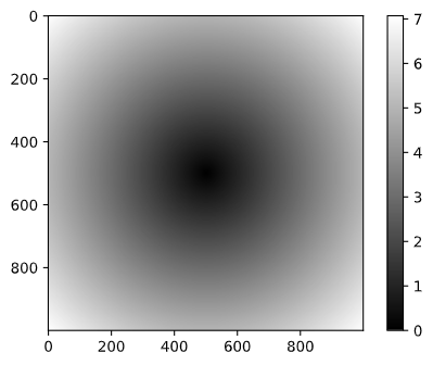
Expressing Conditional Logic as Array Operations
The numpy.where function is a vectorized version of the ternary expression x if condition else y. Suppose we had a boolean array and two arrays of values:
In [26]: xarr = np.array([1.1, 1.2, 1.3, 1.4, 1.5])
In [27]: yarr = np.array([2.1, 2.2, 2.3, 2.4, 2.5])
In [28]: cond = np.array([True, False, True, True, False])
Suppose we wanted to take a value from xarr whenever the corresponding value in cond is True, and otherwise take the value from yarr. A list comprehension doing this might look like:
In [29]: result = [(x if c else y)
         for x, y, c in zip(xarr, yarr, cond)]
In [30]: result
Output: [1.1, 2.2, 1.3, 1.4, 2.5]
This has multiple problems. First, it will not be very fast for large arrays (because all the work is being done in interpreted Python code). Second, it will not work with multidimensional arrays. With np.where you can write this very concisely:
In [31]: result = np.where(cond, xarr, yarr)
In [32]: result
Output: array([ 1.1, 2.2, 1.3, 1.4, 2.5])
The second and third arguments to np.where don’t need to be arrays; one or both of them can be scalars. A typical use of where in data analysis is to produce a new array of values based on another array. Suppose you had a matrix of randomly generated data and you wanted to replace all positive values with 2 and all negative values with –2. This is very easy to do with np.where:
In [33]: arr = np.random.randn(4, 4)
In [34]: arr
Output: array([[-0.44193858,  0.07157006,  2.2441608 , -0.37031764],
       [-0.54374974, -2.62563459,  0.35334962,  1.45375499],
       [-0.09094342,  0.79745038,  0.85707545, -0.6020405 ],
       [-0.61344176, -0.92205991, -0.75273804, -1.69501996]])
In [35]: arr > 0
Output: array([[False,  True,  True, False],
       [False, False,  True,  True],
       [False,  True,  True, False],
       [False, False, False, False]])
In [36]: np.where(arr > 0, 2, -2)
Output: array([[-2,  2,  2, -2],
       [-2, -2,  2,  2],
       [-2,  2,  2, -2],
       [-2, -2, -2, -2]])
You can combine scalars and arrays when using np.where. For example, I can replace all positive values in arr with the constant 2 like so:
In [37]: np.where(arr > 0, 2, arr) # set only positive values to 2
Output: array([[-0.44193858,  2.        ,  2.        , -0.37031764],
       [-0.54374974, -2.62563459,  2.        ,  2.        ],
       [-0.09094342,  2.        ,  2.        , -0.6020405 ],
       [-0.61344176, -0.92205991, -0.75273804, -1.69501996]])
The arrays passed to np.where can be more than just equal-sized arrays or scalars.
